Trace AIC and BIC vs. Penalty

For an ordinary unpenalized fit from lrm, orm, or ols and for a vector or list of penalties, fits a series of logistic or linear models using penalized maximum likelihood estimation, and saves the effective degrees of freedom, Akaike Information Criterion (\(AIC\)), Schwarz Bayesian Information Criterion (\(BIC\)), and Hurvich and Tsai's corrected \(AIC\) (\(AIC_c\)). Optionally pentrace can use the nlminb function to solve for the optimum penalty factor or combination of factors penalizing different kinds of terms in the model. The effective.df function prints the original and effective degrees of freedom for a penalized fit or for an unpenalized fit and the best penalization determined from a previous invocation of pentrace if method="grid" (the default). 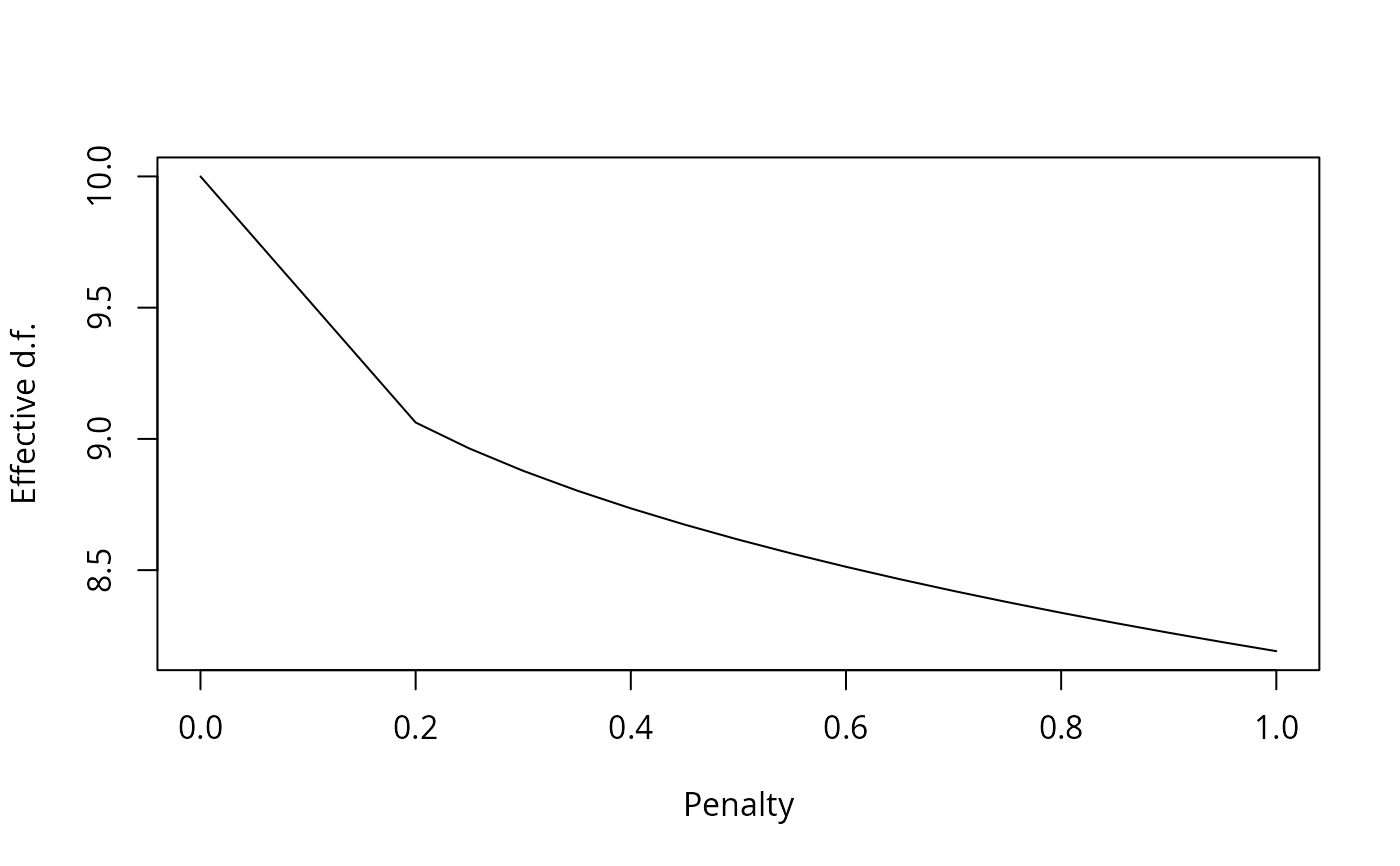The effective d.f. is computed separately for each class of terms in the model (e.g., interaction, nonlinear). 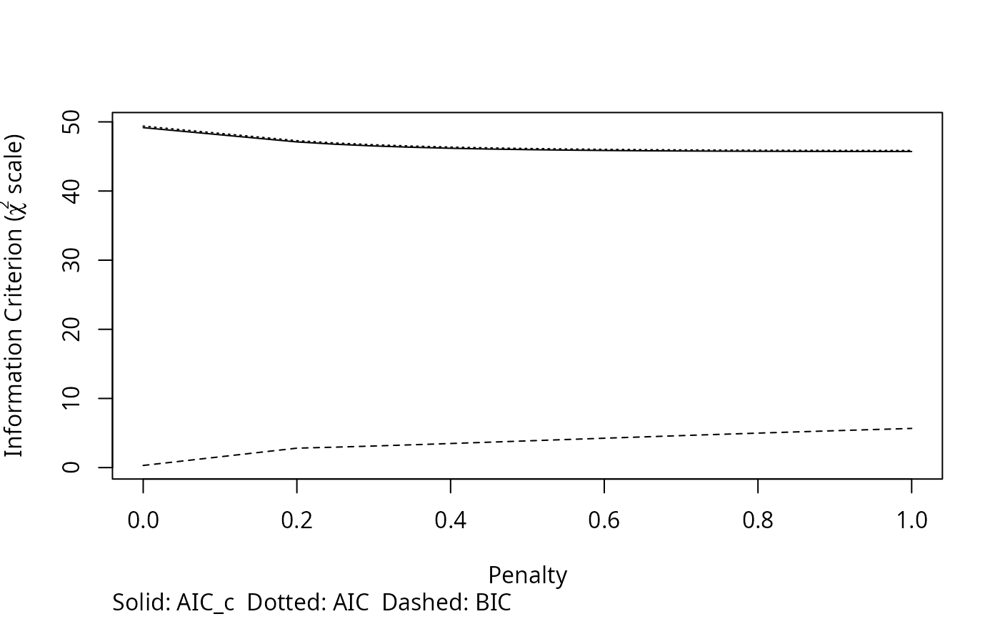A plot method exists to plot the results, and a print method exists to print the most pertinent components. Both \(AIC\) and \(BIC\) may be plotted if there is only one penalty factor type specified in penalty. Otherwise, the first two types of penalty factors are plotted, showing only the \(AIC\).

pentrace(fit, penalty, penalty.matrix, 
         method=c('grid','optimize'),
         which=c('aic.c','aic','bic'), target.df=NULL,
         fitter, pr=FALSE, tol=.Machine$double.eps,
         keep.coef=FALSE, complex.more=TRUE, verbose=FALSE, maxit=20,
         subset, noaddzero=FALSE, ...)

effective.df(fit, object)

# S3 method for class 'pentrace'
print(x, ...)

# S3 method for class 'pentrace'
plot(x, method=c('points','image'), 
     which=c('effective.df','aic','aic.c','bic'), pch=2, add=FALSE, 
     ylim, ...)

Arguments

fit: a result from lrm, orm, or ols with x=TRUE, y=TRUE and without using penalty or penalty.matrix (or optionally using penalization in the case of effective.df)
penalty: can be a vector or a list. If it is a vector, all types of terms in the model will be penalized by the same amount, specified by elements in penalty, with a penalty of zero automatically added. penalty can also be a list in the format documented in the lrm function, except that elements of the list can be vectors. The expand.grid function is invoked by pentrace to generate all possible combinations of penalties. For example, specifying penalty=list(simple=1:2, nonlinear=1:3) will generate 6 combinations to try, so that the analyst can attempt to determine whether penalizing more complex terms in the model more than the linear or categorical variable terms will be beneficial. If complex.more=TRUE, it is assumed that the variables given in penalty are listed in order from less complex to more complex. With method="optimize" penalty specifies an initial guess for the penalty or penalties. If all term types are to be equally penalized, penalty should be a single number, otherwise it should be a list containing single numbers as elements, e.g., penalty=list(simple=1, nonlinear=2). Experience has shown that the optimization algorithm is more likely to find a reasonable solution when the starting value specified in penalty is too large rather than too small.
object: an object returned by pentrace. For effective.df, object can be omitted if the fit was penalized.
penalty.matrix: see lrm
method: The default is method="grid" to print various indexes for all combinations of penalty parameters given by the user. Specify method="optimize" to have pentrace use nlminb to solve for the combination of penalty parameters that gives the maximum value of the objective named in which, or, if target.df is given, to find the combination that yields target.df effective total degrees of freedom for the model. When target.df is specified, method is set to "optimize" automatically. For plot.pentrace this parameter applies only if more than one penalty term-type was used. The default is to use open triangles whose sizes are proportional to the ranks of the AICs, plotting the first two penalty factors respectively on the x and y axes. Use method="image" to plot an image plot.
which: the objective to maximize for either method. Default is "aic.c" (corrected AIC). For plot.pentrace, which is a vector of names of criteria to show; default is to plot all 4 types, with effective d.f. in its own separate plot
target.df: applies only to method="optimize". See method. target.df makes sense mainly when a single type of penalty factor is specified.
fitter: a fitting function. Default is lrm.fit (lm.pfit is always used for ols).
pr: set to TRUE to print intermediate results
tol: tolerance for declaring a matrix singular (see lrm.fit, solvet)
keep.coef: set to TRUE to store matrix of regression coefficients for all the fits (corresponding to increasing values of penalty) in object Coefficients in the returned list. Rows correspond to penalties, columns to regression parameters.
complex.more: By default if penalty is a list, combinations of penalties for which complex terms are penalized less than less complex terms will be dropped after expand.grid is invoked. Set complex.more=FALSE to allow more complex terms to be penalized less. Currently this option is ignored for method="optimize".
verbose: set to TRUE to print number of intercepts and sum of effective degrees of freedom
maxit: maximum number of iterations to allow in a model fit (default=12). This is passed to the appropriate fitter function with the correct argument name. Increase maxit if you had to when fitting the original unpenalized model.
subset: a logical or integer vector specifying rows of the design and response matrices to subset in fitting models. This is most useful for bootstrapping pentrace to see if the best penalty can be estimated with little error so that variation due to selecting the optimal penalty can be safely ignored when bootstrapping standard errors of regression coefficients and measures of predictive accuracy. See an example below.
noaddzero: set to TRUE to not add an unpenalized model to the list of models to fit
x: a result from pentrace
pch: used for method="points"
add: set to TRUE to add to an existing plot. In that case, the effective d.f. plot is not re-drawn, but the AIC/BIC plot is added to.
ylim: 2-vector of y-axis limits for plots other than effective d.f.
...: other arguments passed to plot, lines, or image, or to the fitter

Value

a list of class "pentrace" with elements penalty, df, objective, fit, var.adj, diag, results.all, and optionally Coefficients. The first 6 elements correspond to the fit that had the best objective as named in the which argument, from the sequence of fits tried. Here fit is the fit object from fitter which was a penalized fit, diag is the diagonal of the matrix used to compute the effective d.f., and var.adj is Gray (1992) Equation 2.9, which is an improved covariance matrix for the penalized beta. results.all is a data frame whose first few variables are the components of penalty and whose other columns are df, aic, bic, aic.c. results.all thus contains a summary of results for all fits attempted. When method="optimize", only two components are returned: penalty and objective, and the object does not have a class.

Author

Frank Harrell
Department of Biostatistics
Vanderbilt University
fh@fharrell.com

References

Gray RJ: Flexible methods for analyzing survival data using splines, with applications to breast cancer prognosis. JASA 87:942–951, 1992.

Hurvich CM, Tsai, CL: Regression and time series model selection in small samples. Biometrika 76:297–307, 1989.

Examples

n <- 1000    # define sample size
set.seed(17) # so can reproduce the results
age            <- rnorm(n, 50, 10)
blood.pressure <- rnorm(n, 120, 15)
cholesterol    <- rnorm(n, 200, 25)
sex            <- factor(sample(c('female','male'), n,TRUE))
# Specify population model for log odds that Y=1
L <- .4*(sex=='male') + .045*(age-50) +
  (log(cholesterol - 10)-5.2)*(-2*(sex=='female') + 2*(sex=='male'))
# Simulate binary y to have Prob(y=1) = 1/[1+exp(-L)]
y <- ifelse(runif(n) < plogis(L), 1, 0)


f <- lrm(y ~ blood.pressure + sex * (age + rcs(cholesterol,4)),
         x=TRUE, y=TRUE)
p <- pentrace(f, seq(.2,1,by=.05))
plot(p)


p$diag      # may learn something about fractional effective d.f. 
#> [1] 1
            # for each original parameter
pentrace(f, list(simple=c(0,.2,.4), nonlinear=c(0,.2,.4,.8,1)))
#> 
#> Best penalty:
#> 
#>  simple nonlinear df
#>       0         0 10
#> 
#>  simple nonlinear      df    aic     bic  aic.c
#>     0.0       0.0 10.0000 49.389 0.31126 49.166
#>     0.0       0.2  9.2803 48.315 2.76959 48.122
#>     0.2       0.2  9.0625 47.286 2.81000 47.102
#>     0.0       0.4  8.9605 47.187 3.21069 47.006
#>     0.2       0.4  8.8176 46.673 3.39800 46.498
#>     0.4       0.4  8.7354 46.355 3.48327 46.183
#>     0.0       0.8  8.5771 46.212 4.11762 46.046
#>     0.2       0.8  8.4834 46.092 4.45760 45.930
#>     0.4       0.8  8.4204 46.009 4.68377 45.849
#>     0.0       1.0  8.4391 45.991 4.57354 45.830
#>     0.2       1.0  8.3568 45.949 4.93563 45.791
#>     0.4       1.0  8.2989 45.918 5.18894 45.762


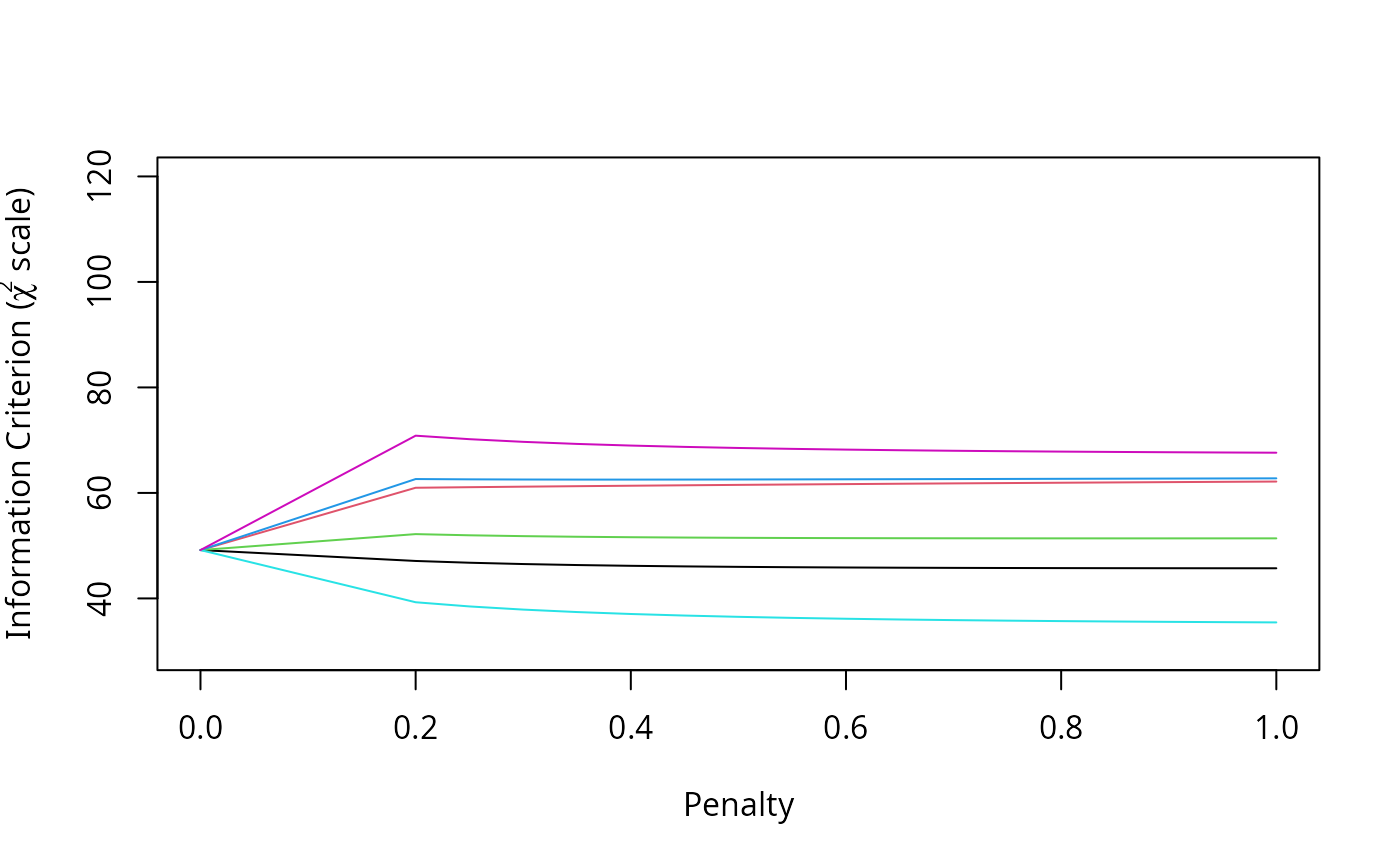
# Bootstrap pentrace 5 times, making a plot of corrected AIC plot with 5 reps
n <- nrow(f$x)
plot(pentrace(f, seq(.2,1,by=.05)), which='aic.c', 
     col=1, ylim=c(30,120)) #original in black
for(j in 1:5)
  plot(pentrace(f, seq(.2,1,by=.05), subset=sample(n,n,TRUE)), 
       which='aic.c', col=j+1, add=TRUE)



# Find penalty giving optimum corrected AIC.  Initial guess is 1.0
# Not implemented yet
# pentrace(f, 1, method='optimize')


# Find penalty reducing total regression d.f. effectively to 5
# pentrace(f, 1, target.df=5)


# Re-fit with penalty giving best aic.c without differential penalization
f <- update(f, penalty=p$penalty)
effective.df(f)
#> 
#> Original and Effective Degrees of Freedom
#> 
#>                          Original Penalized
#> All                            10        10
#> Simple Terms                    4         4
#> Interaction or Nonlinear        6         6
#> Nonlinear                       4         4
#> Interaction                     4         4
#> Nonlinear Interaction           2         2