Brain and Body Weights for 65 Species of Land Animals
Animals2.RdA data frame with average brain and body weights for 62 species of land mammals and three others.
Animals2Format
bodybody weight in kg
brainbrain weight in g
Source
Weisberg, S. (1985) Applied Linear Regression. 2nd edition. Wiley, pp. 144–5.
P. J. Rousseeuw and A. M. Leroy (1987) Robust Regression and Outlier Detection. Wiley, p. 57.
References
Venables, W. N. and Ripley, B. D. (2002) Modern Applied Statistics with S. Forth Edition. Springer.
Note
After loading the MASS package, the data set is simply constructed by
Animals2 <- local({D <- rbind(Animals, mammals);
      unique(D[order(D$body,D$brain),])})
.
Rousseeuw and Leroy (1987)'s ‘brain’ data is the same as
MASS's Animals (with Rat and Brachiosaurus interchanged,
see the example below).
Examples
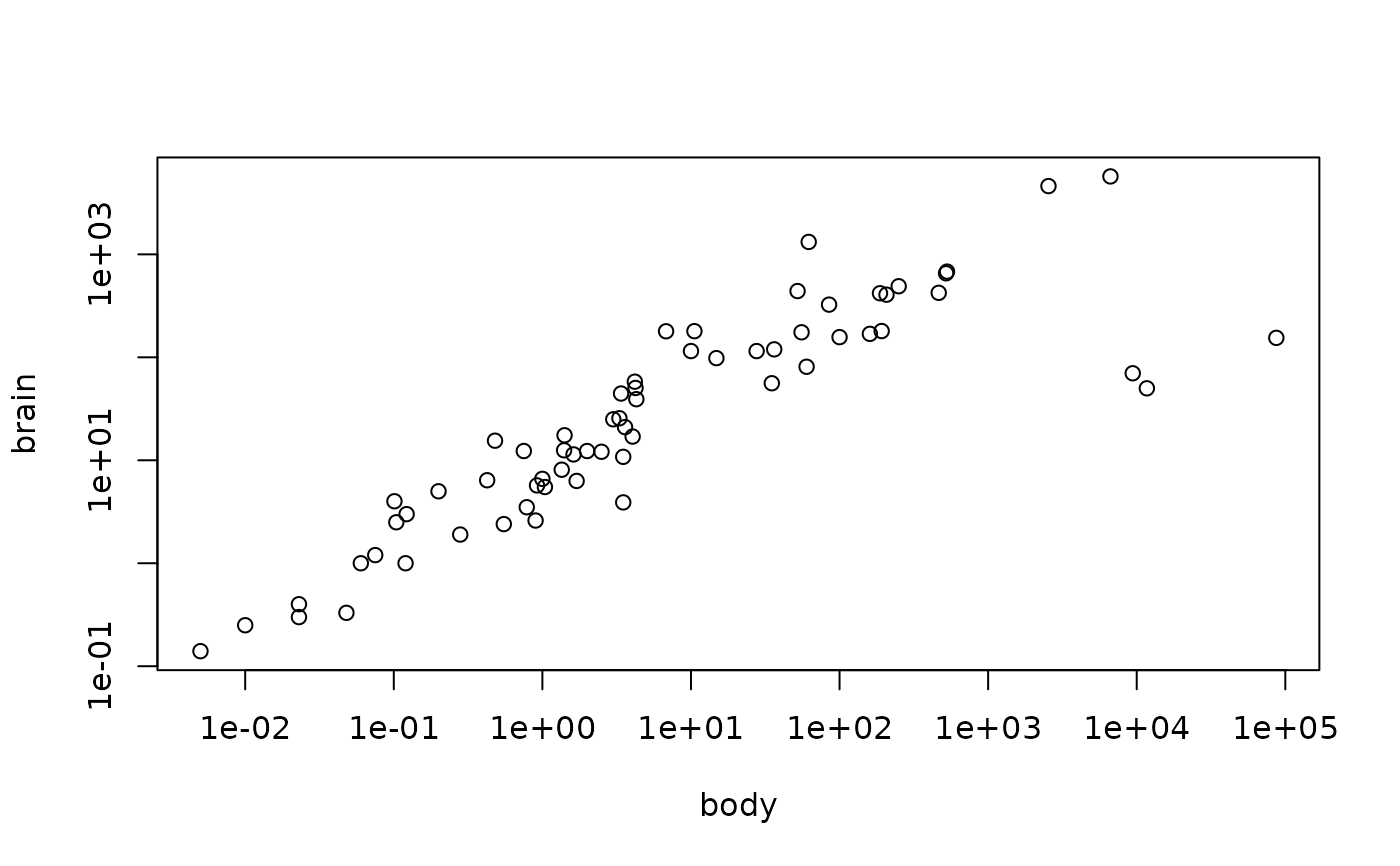
data(Animals2)
## Sensible Plot needs doubly logarithmic scale
plot(Animals2, log = "xy")
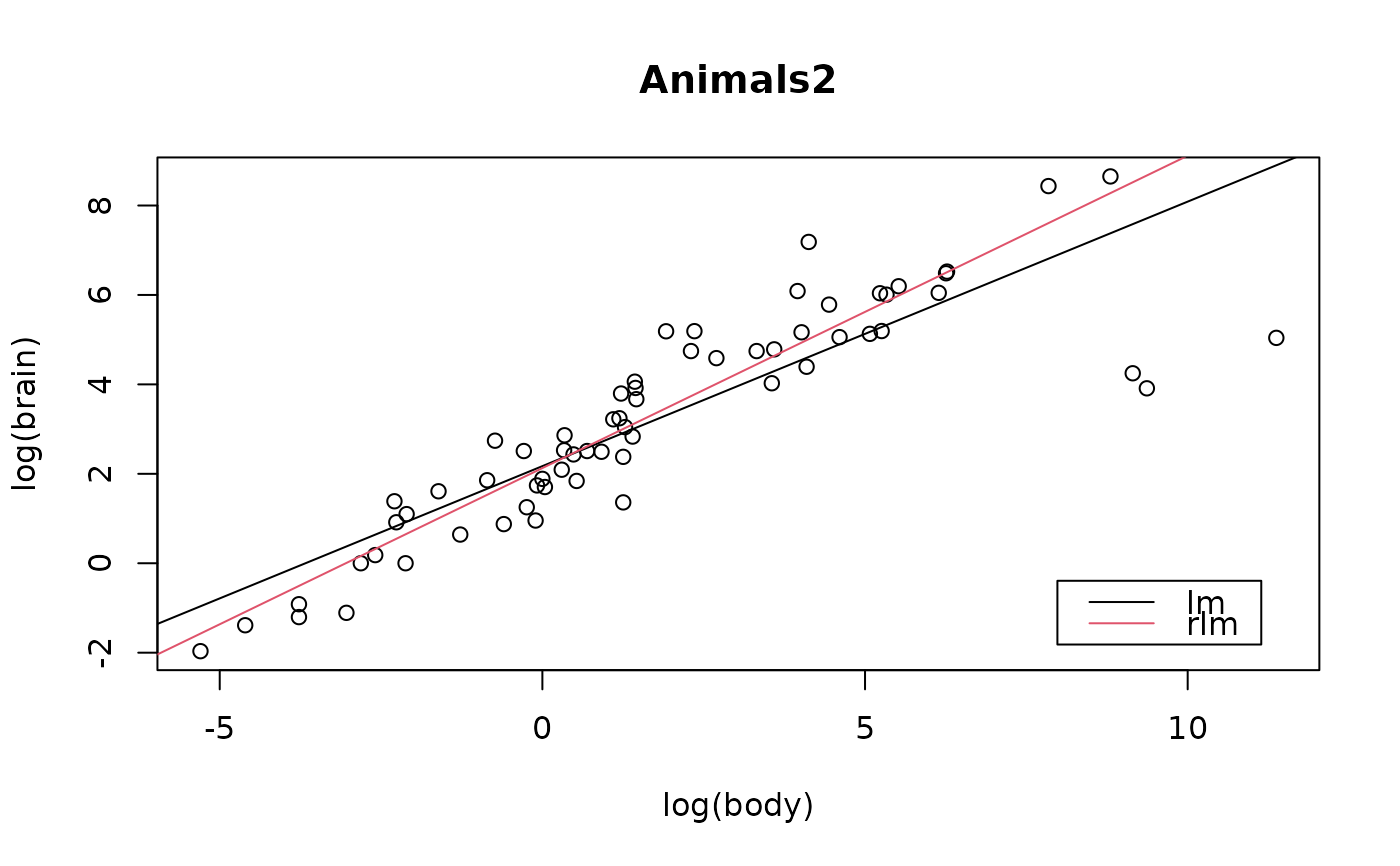
 ## Regression example plot:
plotbb <- function(bbdat) {
d.name <- deparse(substitute(bbdat))
plot(log(brain) ~ log(body), data = bbdat, main = d.name)
abline( lm(log(brain) ~ log(body), data = bbdat))
abline(MASS::rlm(log(brain) ~ log(body), data = bbdat), col = 2)
legend("bottomright", leg = c("lm", "rlm"), col=1:2, lwd=1, inset = 1/20)
}
plotbb(bbdat = Animals2)
## Regression example plot:
plotbb <- function(bbdat) {
d.name <- deparse(substitute(bbdat))
plot(log(brain) ~ log(body), data = bbdat, main = d.name)
abline( lm(log(brain) ~ log(body), data = bbdat))
abline(MASS::rlm(log(brain) ~ log(body), data = bbdat), col = 2)
legend("bottomright", leg = c("lm", "rlm"), col=1:2, lwd=1, inset = 1/20)
}
plotbb(bbdat = Animals2)
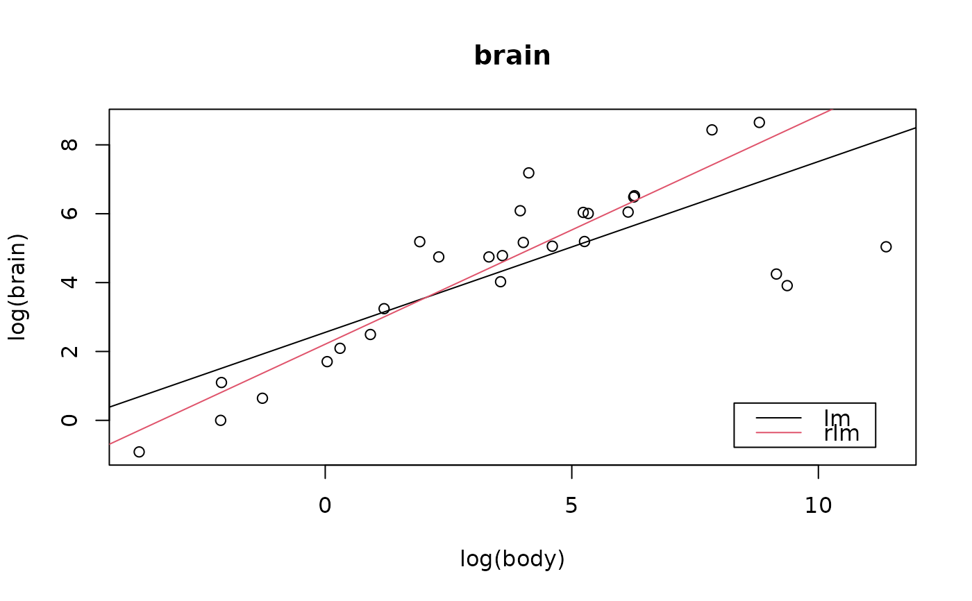
 ## The `same' plot for Rousseeuw's subset:
data(Animals, package = "MASS")
brain <- Animals[c(1:24, 26:25, 27:28),]
plotbb(bbdat = brain)
## The `same' plot for Rousseeuw's subset:
data(Animals, package = "MASS")
brain <- Animals[c(1:24, 26:25, 27:28),]
plotbb(bbdat = brain)
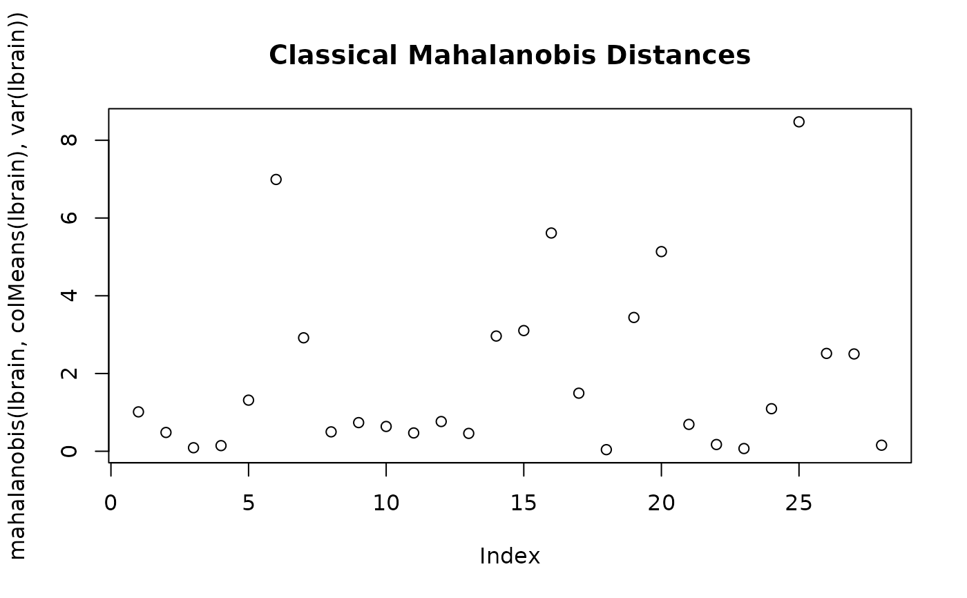
 lbrain <- log(brain)
plot(mahalanobis(lbrain, colMeans(lbrain), var(lbrain)),
main = "Classical Mahalanobis Distances")
lbrain <- log(brain)
plot(mahalanobis(lbrain, colMeans(lbrain), var(lbrain)),
main = "Classical Mahalanobis Distances")
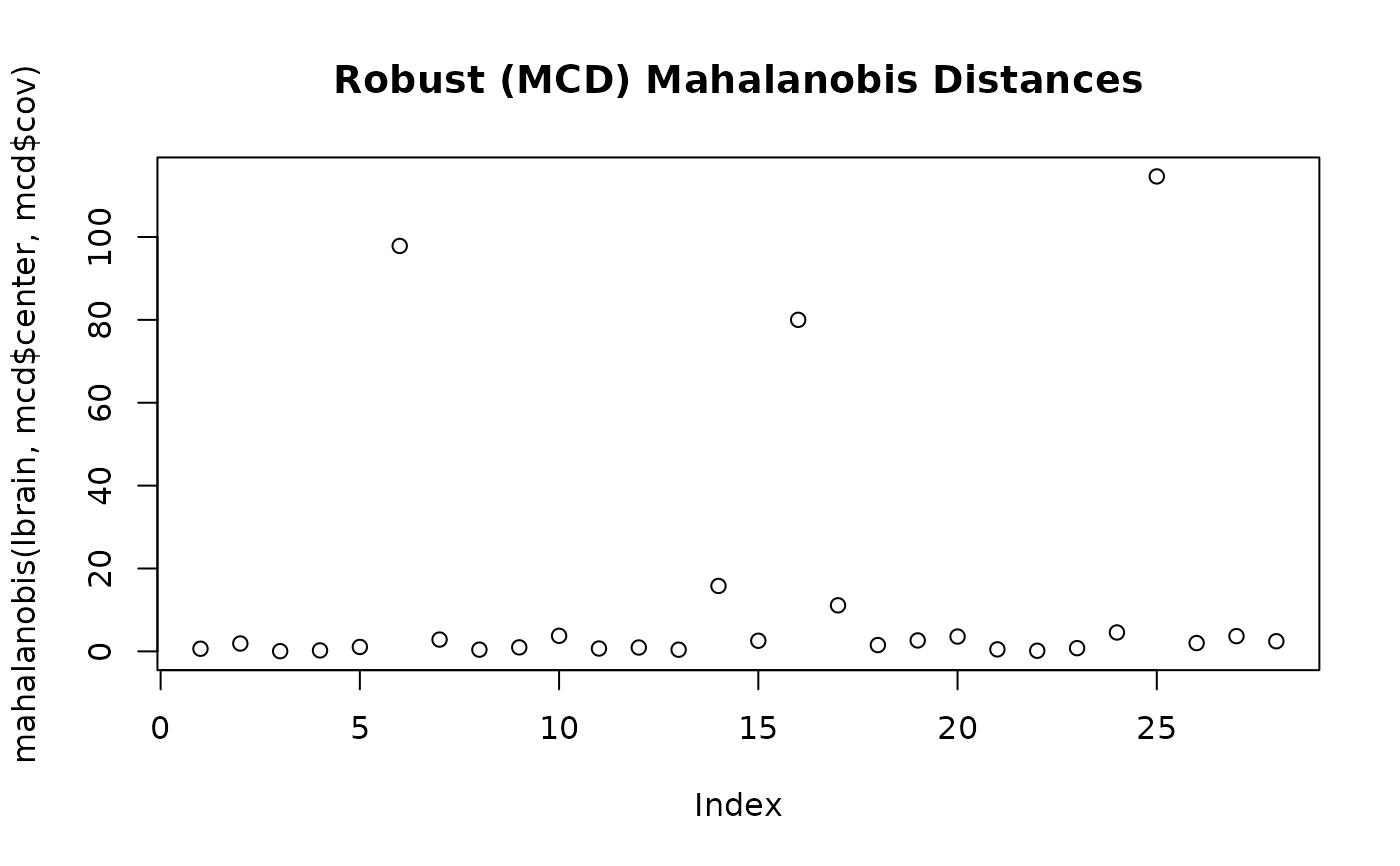
 mcd <- covMcd(lbrain)
plot(mahalanobis(lbrain,mcd$center,mcd$cov),
main = "Robust (MCD) Mahalanobis Distances")
mcd <- covMcd(lbrain)
plot(mahalanobis(lbrain,mcd$center,mcd$cov),
main = "Robust (MCD) Mahalanobis Distances")