Robust Location-Free Scale Estimate More Efficient than MAD

Compute the robust scale estimator \(Q_n\), an efficient alternative to the MAD.

By default, \(Q_n(x_1, \ldots, x_n)\) is the \(k\)-th order statistic (a quantile) of the choose(n, 2) absolute differences \(|x_i - x_j|\), (for \(1 \le i < j \le n\)), where by default (originally only possible value) \(k = choose(n\%/\% 2 + 1, 2)\) which is about the first quartile (25% quantile) of these pairwise differences. See the references for more.

Qn(x, constant = NULL, finite.corr = is.null(constant) && missing(k),
   na.rm = FALSE, k = choose(n %/% 2 + 1, 2), warn.finite.corr = TRUE)

s_Qn(x, mu.too = FALSE, ...)

Arguments

x

numeric vector of observations.

constant

number by which the result is multiplied; the default achieves consistency for normally distributed data. Note that until Nov. 2010, “thanks” to a typo in the very first papers, a slightly wrong default constant, 2.2219, was used instead of the correct one which is equal to 1 / (sqrt(2) * qnorm(5/8)) (as mentioned already on p.1277, after (3.7) in Rousseeuw and Croux (1993)).

If you need the old slightly off version for historical reproducibility, you can use Qn.old().

Note that the relative difference is only about 1 in 1000, and that the correction should not affect the finite sample corrections for \(n \le 9\).

finite.corr

logical indicating if the finite sample bias correction factor should be applied. Defaults to TRUE unless constant is specified. Note the for non-default k, the consistency constant already depends on n leading to some finite sample correction, but no simulation-based small-n correction factors are available.

na.rm

logical specifying if missing values (NA) should be removed from x before further computation. If false as by default, and if there are NAs, i.e., if(anyNA(x)), the result will be NA.

k

integer, typically half of n, specifying the “quantile”, i.e., rather the order statistic that Qn() should return; for the Qn() proper, this has been hard wired to choose(n%/%2 +1, 2), i.e., \(\lfloor\frac{n}{2}\rfloor +1\). Choosing a large k is less robust but allows to get non-zero results in case the default Qn() is zero.

warn.finite.corr

logical indicating if a warning should be signalled when k is non-default, in which case specific small-\(n\) correction is not yet provided.

mu.too

logical indicating if the median(x) should also be returned for s_Qn().

...

potentially further arguments for s_Qn() passed to Qn().

Value

Qn() returns a number, the \(Q_n\) robust scale estimator, scaled to be consistent for \(\sigma^2\) and i.i.d. Gaussian observations, optionally bias corrected for finite samples.

s_Qn(x, mu.too=TRUE) returns a length-2 vector with location (\(\mu\)) and scale; this is typically only useful for covOGK(*, sigmamu = s_Qn).

Details

As the (default, consistency) constant needed to be corrected, the finite sample correction has been based on a much more extensive simulation, and on a 3rd or 4th degree polynomial model in \(1/n\) for odd or even n, respectively.

References

Rousseeuw, P.J. and Croux, C. (1993) Alternatives to the Median Absolute Deviation, Journal of the American Statistical Association 88, 1273–1283. doi:10.2307/2291267

Christophe Croux and Peter J. Rousseeuw (1992) A class of high-breakdown scale estimators based on subranges , Communications in Statistics - Theory and Methods 21, 1935–1951; doi:10.1080/03610929208830889

Christophe Croux and Peter J. Rousseeuw (1992) Time-Efficient Algorithms for Two Highly Robust Estimators of Scale, Computational Statistics, Vol. 1, ed. Dodge and Whittaker, Physica-Verlag Heidelberg, 411–428; available via Springer Link.

About the typo in the constant:
Christophe Croux (2010) Private e-mail, Fri Jul 16, w/ Subject Re: Slight inaccuracy of Qn implementation .......

Author

Original Fortran code: Christophe Croux and Peter Rousseeuw rousse@wins.uia.ac.be.
Port to C and R: Martin Maechler, maechler@R-project.org

Examples

set.seed(153)
x <- sort(c(rnorm(80), rt(20, df = 1)))
s_Qn(x, mu.too = TRUE)
#> [1] -0.2154659  1.1766966
Qn(x, finite.corr = FALSE)
#> [1] 1.220186

## A simple pure-R version of Qn() -- slow and memory-rich for large n: O(n^2)
Qn0R <- function(x, k = choose(n %/% 2 + 1, 2)) { 
    n <- length(x <- sort(x))
    if(n == 0) return(NA) else if(n == 1) return(0.)
    stopifnot(is.numeric(k), k == as.integer(k), 1 <= k, k <= n*(n-1)/2)
    m <- outer(x,x,"-")# abs not needed as x[] is sorted
    sort(m[lower.tri(m)], partial = k)[k]
}
(Qx1 <- Qn(x, constant=1)) # 0.5498463
#> [1] 0.5498463
## the C-algorithm "rounds" to 'float' single precision ..
stopifnot(all.equal(Qx1, Qn0R(x), tol = 1e-6))


(qn <- Qn(c(1:4, 10, Inf, NA), na.rm=TRUE))
#> [1] 4.075673
stopifnot(is.finite(qn), all.equal(4.075672524, qn, tol=1e-10))

## -- compute for different 'k' :

n <- length(x) # = 100 here
(k0 <- choose(floor(n/2) + 1, 2)) # 51*50/2 == 1275
#> [1] 1275
stopifnot(identical(Qx1, Qn(x, constant=1, k=k0)))
nn2 <- n*(n-1)/2
all.k <- 1:nn2
system.time(Qss <- sapply(all.k, function(k) Qn(x, 1, k=k)))
#>    user  system elapsed 
#>   0.098   0.000   0.099 
system.time(Qs  <- Qn  (x, 1, k = all.k))
#>    user  system elapsed 
#>    0.05    0.00    0.05 
system.time(Qs0 <- Qn0R(x,    k = all.k) )
#>    user  system elapsed 
#>   0.001   0.000   0.001 
stopifnot(exprs = {
   Qs[1]   == min(diff(x))
   Qs[nn2] == diff(range(x))
   all.equal(Qs,  Qss, tol = 1e-15) # even exactly
   all.equal(Qs0, Qs, tol = 1e-7) # see 2.68e-8, as Qn() C-code rounds to (float)
})

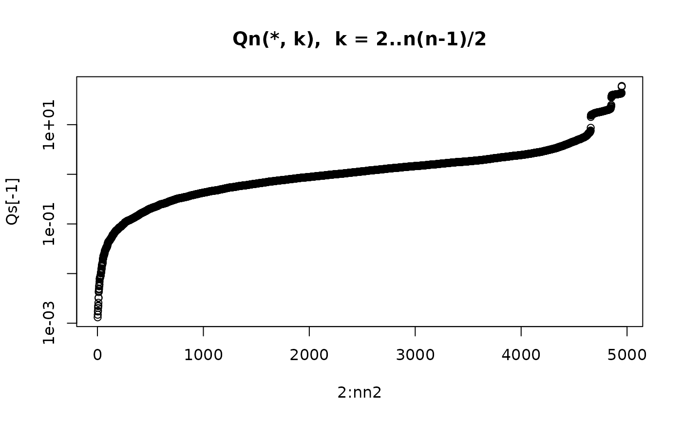
plot(2:nn2, Qs[-1], type="b", log="y", main = "Qn(*, k),  k = 2..n(n-1)/2")