Coleman Data Set

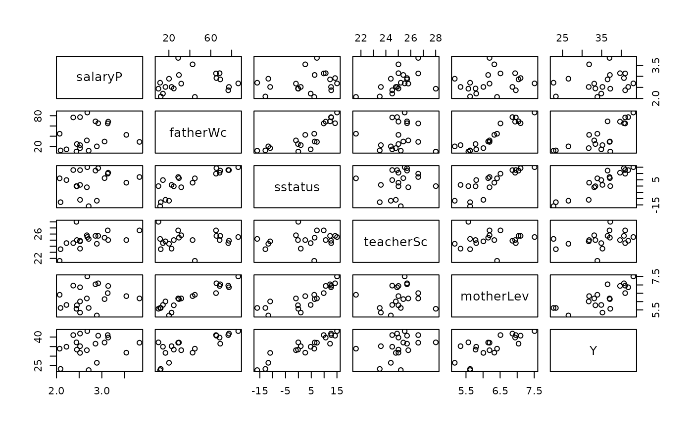
Contains information on 20 Schools from the Mid-Atlantic and New England States, drawn from a population studied by Coleman et al. (1966). Mosteller and Tukey (1977) analyze this sample consisting of measurements on six different variables, one of which will be treated as a responce.

data(coleman, package="robustbase")

Format

A data frame with 20 observations on the following 6 variables.

salaryP

staff salaries per pupil

fatherWc

percent of white-collar fathers

sstatus

socioeconomic status composite deviation: means for family size, family intactness, father's education, mother's education, and home items

teacherSc

mean teacher's verbal test score

motherLev

mean mother's educational level, one unit is equal to two school years

Y

verbal mean test score (y, all sixth graders)

Author

Valentin Todorov

Source

P. J. Rousseeuw and A. M. Leroy (1987) Robust Regression and Outlier Detection Wiley, p.79, table 2.

Examples

data(coleman)
pairs(coleman)

summary( lm.coleman <-     lm(Y ~ . , data = coleman))
#> 
#> Call:
#> lm(formula = Y ~ ., data = coleman)
#> 
#> Residuals:
#>     Min      1Q  Median      3Q     Max 
#> -3.9497 -0.6174  0.0623  0.7343  5.0018 
#> 
#> Coefficients:
#>             Estimate Std. Error t value Pr(>|t|)    
#> (Intercept) 19.94857   13.62755   1.464   0.1653    
#> salaryP     -1.79333    1.23340  -1.454   0.1680    
#> fatherWc     0.04360    0.05326   0.819   0.4267    
#> sstatus      0.55576    0.09296   5.979 3.38e-05 ***
#> teacherSc    1.11017    0.43377   2.559   0.0227 *  
#> motherLev   -1.81092    2.02739  -0.893   0.3868    
#> ---
#> Signif. codes:  0 ‘***’ 0.001 ‘**’ 0.01 ‘*’ 0.05 ‘.’ 0.1 ‘ ’ 1
#> 
#> Residual standard error: 2.074 on 14 degrees of freedom
#> Multiple R-squared:  0.9063,	Adjusted R-squared:  0.8728 
#> F-statistic: 27.08 on 5 and 14 DF,  p-value: 9.927e-07
#> 
summary(lts.coleman <- ltsReg(Y ~ . , data = coleman))
#> 
#> Call:
#> ltsReg.formula(formula = Y ~ ., data = coleman)
#> 
#> Residuals (from reweighted LS):
#>     Min      1Q  Median      3Q     Max 
#> -1.2155 -0.3887  0.0000  0.3056  0.9845 
#> 
#> Coefficients:
#>           Estimate Std. Error t value Pr(>|t|)    
#> Intercept 29.75772    5.53224   5.379 0.000166 ***
#> salaryP   -1.69854    0.46602  -3.645 0.003358 ** 
#> fatherWc   0.08512    0.02079   4.093 0.001490 ** 
#> sstatus    0.66617    0.03824  17.423 6.94e-10 ***
#> teacherSc  1.18400    0.16425   7.208 1.07e-05 ***
#> motherLev -4.06675    0.84867  -4.792 0.000440 ***
#> ---
#> Signif. codes:  0 ‘***’ 0.001 ‘**’ 0.01 ‘*’ 0.05 ‘.’ 0.1 ‘ ’ 1
#> 
#> Residual standard error: 0.7824 on 12 degrees of freedom
#> Multiple R-Squared: 0.9883,	Adjusted R-squared: 0.9835 
#> F-statistic: 203.2 on 5 and 12 DF,  p-value: 3.654e-11 
#> 

coleman.x <- data.matrix(coleman[, 1:6])
(Cc <- covMcd(coleman.x))
#> Minimum Covariance Determinant (MCD) estimator approximation.
#> Method: Fast MCD(alpha=0.5 ==> h=13); nsamp = 500; (n,k)mini = (300,5)
#> Call:
#> covMcd(x = coleman.x)
#> Log(Det.):  1.558 
#> 
#> Robust Estimate of Location:
#>   salaryP   fatherWc    sstatus  teacherSc  motherLev          Y  
#>     2.615     43.302      2.805     24.766      6.271     34.733  
#> Robust Estimate of Covariance:
#>            salaryP  fatherWc  sstatus  teacherSc  motherLev        Y
#> salaryP    0.35626     6.383    1.469     0.8384    0.09473    1.795
#> fatherWc   6.38271  1990.496  638.056    18.3330   45.27247  431.265
#> sstatus    1.46861   638.056  283.812     5.5912   15.94033  184.824
#> teacherSc  0.83836    18.333    5.591     3.7826    0.37961    6.997
#> motherLev  0.09473    45.272   15.940     0.3796    1.16723   10.396
#> Y          1.79545   431.265  184.824     6.9968   10.39554  124.221