Example Data of Antille and May - for Simple Regression

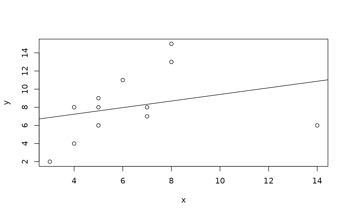
This is an artificial data set, cleverly construced and used by Antille and May to demonstrate ‘problems’ with LMS and LTS.

data(exAM, package="robustbase")

Format

A data frame with 12 observations on 2 variables, x and y.

Details

Because the points are not in general position, both LMS and LTS typically fail; however, e.g., rlm(*, method="MM") “works”.

Source

Antille, G. and El May, H. (1992) The use of slices in the LMS and the method of density slices: Foundation and comparison.
In Yadolah Dodge and Joe Whittaker, editors, COMPSTAT: Proc. 10th Symp. Computat. Statist., Neuchatel, 1, 441–445; Physica-Verlag.

Examples

data(exAM)
plot(exAM)
summary(ls <- lm(y ~ x, data=exAM))
#> 
#> Call:
#> lm(formula = y ~ x, data = exAM)
#> 
#> Residuals:
#>     Min      1Q  Median      3Q     Max 
#> -4.8723 -2.0081  0.0378  1.8103  6.3112 
#> 
#> Coefficients:
#>             Estimate Std. Error t value Pr(>|t|)  
#> (Intercept)   5.7824     2.6171   2.209   0.0516 .
#> x             0.3633     0.3784   0.960   0.3596  
#> ---
#> Signif. codes:  0 ‘***’ 0.001 ‘**’ 0.01 ‘*’ 0.05 ‘.’ 0.1 ‘ ’ 1
#> 
#> Residual standard error: 3.643 on 10 degrees of freedom
#> Multiple R-squared:  0.0844,	Adjusted R-squared:  -0.007157 
#> F-statistic: 0.9218 on 1 and 10 DF,  p-value: 0.3596
#> 
abline(ls)