Heart Catherization Data

This data set was analyzed by Weisberg (1980) and Chambers et al. (1983). A catheter is passed into a major vein or artery at the femoral region and moved into the heart. The proper length of the introduced catheter has to be guessed by the physician. The aim of the data set is to describe the relation between the catheter length and the patient's height (X1) and weight (X2).

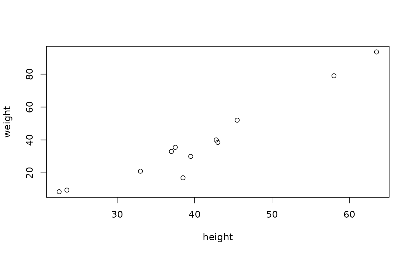
This data sets is used to demonstrate the effects caused by collinearity. The correlation between height and weight is so high that either variable almost completely determines the other.

data(heart)
<!-- %&gt; QA bug: would want: -->
<!-- %&gt; data(heart, package="robustbase") -->
<!-- %&gt; but that gives two warnings -->

Format

A data frame with 12 observations on the following 3 variables.

height

Patient's height in inches

weight

Patient's weights in pounds

clength

Y: Catheter Length (in centimeters)

Note

There are other heart datasets in other R packages, notably survival, hence considering using package = "robustbase", see examples.

Source

Weisberg (1980)

Chambers et al. (1983)

P. J. Rousseeuw and A. M. Leroy (1987) Robust Regression and Outlier Detection; Wiley, p.103, table 13.

Examples

data(heart, package="robustbase")
heart.x <- data.matrix(heart[, 1:2]) # the X-variables
plot(heart.x)

covMcd(heart.x)
#> Minimum Covariance Determinant (MCD) estimator approximation.
#> Method: Fast MCD(alpha=0.5 ==> h=7); nsamp = 500; (n,k)mini = (300,5)
#> Call:
#> covMcd(x = heart.x)
#> Log(Det.):  5.679 
#> 
#> Robust Estimate of Location:
#> height  weight  
#>  38.25   33.09  
#> Robust Estimate of Covariance:
#>         height  weight
#> height   134.5   258.7
#> weight   258.7   564.4
summary( lm.heart <-     lm(clength ~ . , data = heart))
#> 
#> Call:
#> lm(formula = clength ~ ., data = heart)
#> 
#> Residuals:
#>     Min      1Q  Median      3Q     Max 
#> -6.7419 -1.2034 -0.2595  1.8892  6.6566 
#> 
#> Coefficients:
#>             Estimate Std. Error t value Pr(>|t|)  
#> (Intercept)  20.3758     8.3859   2.430    0.038 *
#> height        0.2107     0.3455   0.610    0.557  
#> weight        0.1911     0.1583   1.207    0.258  
#> ---
#> Signif. codes:  0 ‘***’ 0.001 ‘**’ 0.01 ‘*’ 0.05 ‘.’ 0.1 ‘ ’ 1
#> 
#> Residual standard error: 3.778 on 9 degrees of freedom
#> Multiple R-squared:  0.8254,	Adjusted R-squared:  0.7865 
#> F-statistic: 21.27 on 2 and 9 DF,  p-value: 0.0003888
#> 
summary(lts.heart <- ltsReg(clength ~ . , data = heart))
#> 
#> Call:
#> ltsReg.formula(formula = clength ~ ., data = heart)
#> 
#> Residuals (from reweighted LS):
#>       1       2       3       4       5       6       7       8       9      10 
#> -1.3927  0.1691  0.0000  0.4434 -0.3413  0.1655 -0.1148  0.0000  0.0000  0.0000 
#>      11      12 
#>  0.6663  0.4045 
#> 
#> Coefficients:
#>           Estimate Std. Error t value Pr(>|t|)    
#> Intercept 63.35284    4.02270  15.749 1.88e-05 ***
#> height    -1.22650    0.14032  -8.741 0.000325 ***
#> weight     0.68835    0.05278  13.041 4.73e-05 ***
#> ---
#> Signif. codes:  0 ‘***’ 0.001 ‘**’ 0.01 ‘*’ 0.05 ‘.’ 0.1 ‘ ’ 1
#> 
#> Residual standard error: 0.7654 on 5 degrees of freedom
#> Multiple R-Squared: 0.9913,	Adjusted R-squared: 0.9879 
#> F-statistic:   286 on 2 and 5 DF,  p-value: 6.992e-06 
#>