Modified Data on Wood Specific Gravity
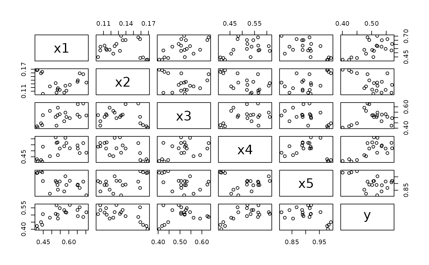
wood.RdThe original data are from Draper and Smith (1966) and were used to determine the influence of anatomical factors on wood specific gravity, with five explanatory variables and an intercept. These data were contaminated by replacing a few observations with outliers.
data(wood, package="robustbase")Format
A data frame with 20 observations on the following 6 variables.
- x1, x2, x3, x4, x5
explanatory “anatomical” wood variables.
- y
wood specific gravity, the target variable.
Source
Draper and Smith (1966, p.227)
Peter J. Rousseeuw and Annick M. Leroy (1987) Robust Regression and Outlier Detection Wiley, p.243, table 8.
Examples
data(wood)
plot(wood)

summary( lm.wood <-        lm(y ~ ., data = wood))
#>
#> Call:
#> lm(formula = y ~ ., data = wood)
#>
#> Residuals:
#>       Min        1Q    Median        3Q       Max
#> -0.030415 -0.012318 -0.003494  0.012760  0.047892
#>
#> Coefficients:
#>             Estimate Std. Error t value Pr(>|t|)
#> (Intercept)  0.42178    0.16912   2.494  0.02576 *
#> x1           0.44069    0.11688   3.770  0.00207 **
#> x2          -1.47501    0.48692  -3.029  0.00901 **
#> x3          -0.26118    0.11199  -2.332  0.03513 *
#> x4           0.02079    0.16109   0.129  0.89915
#> x5           0.17082    0.20336   0.840  0.41505
#> ---
#> Signif. codes:  0 ‘***’ 0.001 ‘**’ 0.01 ‘*’ 0.05 ‘.’ 0.1 ‘ ’ 1
#>
#> Residual standard error: 0.02412 on 14 degrees of freedom
#> Multiple R-squared:  0.8084,	Adjusted R-squared:   0.74
#> F-statistic: 11.81 on 5 and 14 DF,  p-value: 0.0001282
#>
summary(rlm.wood <- MASS::rlm(y ~ ., data = wood))
#>
#> Call: rlm(formula = y ~ ., data = wood)
#> Residuals:
#>       Min        1Q    Median        3Q       Max
#> -0.029872 -0.011744 -0.002467  0.012984  0.058431
#>
#> Coefficients:
#>             Value   Std. Error t value
#> (Intercept)  0.3986  0.1673     2.3823
#> x1           0.4124  0.1156     3.5661
#> x2          -1.6204  0.4817    -3.3638
#> x3          -0.2288  0.1108    -2.0652
#> x4           0.0202  0.1594     0.1268
#> x5           0.2152  0.2012     1.0695
#>
#> Residual standard error: 0.0193 on 14 degrees of freedom
summary(lts.wood <-    ltsReg(y ~ ., data = wood))
#>
#> Call:
#> ltsReg.formula(formula = y ~ ., data = wood)
#>
#> Residuals (from reweighted LS):
#>       Min        1Q    Median        3Q       Max
#> -0.009281 -0.001771  0.000000  0.001146  0.013004
#>
#> Coefficients:
#>           Estimate Std. Error t value Pr(>|t|)
#> Intercept  0.37733    0.05402   6.986 3.78e-05 ***
#> x1         0.21738    0.04212   5.162 0.000424 ***
#> x2        -0.08501    0.19771  -0.430 0.676341
#> x3        -0.56430    0.04349 -12.975 1.40e-07 ***
#> x4        -0.40033    0.06544  -6.118 0.000113 ***
#> x5         0.60745    0.07858   7.730 1.59e-05 ***
#> ---
#> Signif. codes:  0 ‘***’ 0.001 ‘**’ 0.01 ‘*’ 0.05 ‘.’ 0.1 ‘ ’ 1
#>
#> Residual standard error: 0.007451 on 10 degrees of freedom
#> Multiple R-Squared: 0.9583,	Adjusted R-squared: 0.9375
#> F-statistic:    46 on 5 and 10 DF,  p-value: 1.397e-06
#>

wood.x <- as.matrix(wood)[,1:5]
c_wood <- covMcd(wood.x)
c_wood
#> Minimum Covariance Determinant (MCD) estimator approximation.
#> Method: Fast MCD(alpha=0.5 ==> h=13); nsamp = 500; (n,k)mini = (300,5)
#> Call:
#> covMcd(x = wood.x)
#> Log(Det.):  -36.27
#>
#> Robust Estimate of Location:
#>     x1      x2      x3      x4      x5
#> 0.5869  0.1222  0.5309  0.5382  0.8918
#> Robust Estimate of Covariance:
#>             x1          x2          x3          x4          x5
#> x1   0.0100246   1.881e-03   0.0031533  -5.859e-04  -1.630e-03
#> x2   0.0018808   4.847e-04   0.0012691  -5.199e-05   2.364e-05
#> x3   0.0031533   1.269e-03   0.0066322  -8.713e-04   3.524e-04
#> x4  -0.0005859  -5.199e-05  -0.0008713   2.846e-03   1.828e-03
#> x5  -0.0016299   2.364e-05   0.0003524   1.828e-03   2.767e-03
summary( lm.wood <- lm(y ~ ., data = wood))
#>
#> Call:
#> lm(formula = y ~ ., data = wood)
#>
#> Residuals:
#> Min 1Q Median 3Q Max
#> -0.030415 -0.012318 -0.003494 0.012760 0.047892
#>
#> Coefficients:
#> Estimate Std. Error t value Pr(>|t|)
#> (Intercept) 0.42178 0.16912 2.494 0.02576 *
#> x1 0.44069 0.11688 3.770 0.00207 **
#> x2 -1.47501 0.48692 -3.029 0.00901 **
#> x3 -0.26118 0.11199 -2.332 0.03513 *
#> x4 0.02079 0.16109 0.129 0.89915
#> x5 0.17082 0.20336 0.840 0.41505
#> ---
#> Signif. codes: 0 ‘***’ 0.001 ‘**’ 0.01 ‘*’ 0.05 ‘.’ 0.1 ‘ ’ 1
#>
#> Residual standard error: 0.02412 on 14 degrees of freedom
#> Multiple R-squared: 0.8084, Adjusted R-squared: 0.74
#> F-statistic: 11.81 on 5 and 14 DF, p-value: 0.0001282
#>
summary(rlm.wood <- MASS::rlm(y ~ ., data = wood))
#>
#> Call: rlm(formula = y ~ ., data = wood)
#> Residuals:
#> Min 1Q Median 3Q Max
#> -0.029872 -0.011744 -0.002467 0.012984 0.058431
#>
#> Coefficients:
#> Value Std. Error t value
#> (Intercept) 0.3986 0.1673 2.3823
#> x1 0.4124 0.1156 3.5661
#> x2 -1.6204 0.4817 -3.3638
#> x3 -0.2288 0.1108 -2.0652
#> x4 0.0202 0.1594 0.1268
#> x5 0.2152 0.2012 1.0695
#>
#> Residual standard error: 0.0193 on 14 degrees of freedom
summary(lts.wood <- ltsReg(y ~ ., data = wood))
#>
#> Call:
#> ltsReg.formula(formula = y ~ ., data = wood)
#>
#> Residuals (from reweighted LS):
#> Min 1Q Median 3Q Max
#> -0.009281 -0.001771 0.000000 0.001146 0.013004
#>
#> Coefficients:
#> Estimate Std. Error t value Pr(>|t|)
#> Intercept 0.37733 0.05402 6.986 3.78e-05 ***
#> x1 0.21738 0.04212 5.162 0.000424 ***
#> x2 -0.08501 0.19771 -0.430 0.676341
#> x3 -0.56430 0.04349 -12.975 1.40e-07 ***
#> x4 -0.40033 0.06544 -6.118 0.000113 ***
#> x5 0.60745 0.07858 7.730 1.59e-05 ***
#> ---
#> Signif. codes: 0 ‘***’ 0.001 ‘**’ 0.01 ‘*’ 0.05 ‘.’ 0.1 ‘ ’ 1
#>
#> Residual standard error: 0.007451 on 10 degrees of freedom
#> Multiple R-Squared: 0.9583, Adjusted R-squared: 0.9375
#> F-statistic: 46 on 5 and 10 DF, p-value: 1.397e-06
#>
wood.x <- as.matrix(wood)[,1:5]
c_wood <- covMcd(wood.x)
c_wood
#> Minimum Covariance Determinant (MCD) estimator approximation.
#> Method: Fast MCD(alpha=0.5 ==> h=13); nsamp = 500; (n,k)mini = (300,5)
#> Call:
#> covMcd(x = wood.x)
#> Log(Det.): -36.27
#>
#> Robust Estimate of Location:
#> x1 x2 x3 x4 x5
#> 0.5869 0.1222 0.5309 0.5382 0.8918
#> Robust Estimate of Covariance:
#> x1 x2 x3 x4 x5
#> x1 0.0100246 1.881e-03 0.0031533 -5.859e-04 -1.630e-03
#> x2 0.0018808 4.847e-04 0.0012691 -5.199e-05 2.364e-05
#> x3 0.0031533 1.269e-03 0.0066322 -8.713e-04 3.524e-04
#> x4 -0.0005859 -5.199e-05 -0.0008713 2.846e-03 1.828e-03
#> x5 -0.0016299 2.364e-05 0.0003524 1.828e-03 2.767e-03