Plot method for model parameters

The plot() method for the parameters::model_parameters() function.

# S3 method for class 'see_parameters_model'
plot(
  x,
  show_intercept = FALSE,
  size_point = 0.8,
  size_text = NA,
  sort = NULL,
  n_columns = NULL,
  type = c("forest", "funnel"),
  weight_points = TRUE,
  show_labels = FALSE,
  show_estimate = TRUE,
  show_interval = TRUE,
  show_density = FALSE,
  show_direction = TRUE,
  log_scale = FALSE,
  ...
)

# S3 method for class 'see_parameters_sem'
plot(
  x,
  data = NULL,
  component = c("regression", "correlation", "loading"),
  type = component,
  threshold_coefficient = NULL,
  threshold_p = NULL,
  ci = TRUE,
  size_point = 22,
  ...
)

Arguments

x

An object.

show_intercept

Logical, if TRUE, the intercept-parameter is included in the plot. By default, it is hidden because in many cases the intercept-parameter has a posterior distribution on a very different location, so density curves of posterior distributions for other parameters are hardly visible.

size_point

Numeric specifying size of point-geoms.

size_text

Numeric value specifying size of text labels.

sort

The behavior of this argument depends on the plotting contexts.

• Plotting model parameters: If NULL, coefficients are plotted in the order as they appear in the summary. Setting sort = "ascending" or sort = "descending" sorts coefficients in ascending or descending order, respectively. Setting sort = TRUE is the same as sort = "ascending".

• Plotting Bayes factors: Sort pie-slices by posterior probability (descending)?

n_columns

For models with multiple components (like fixed and random, count and zero-inflated), defines the number of columns for the panel-layout. If NULL, a single, integrated plot is shown.

type

Character indicating the type of plot. Only applies for model parameters from meta-analysis objects (e.g. metafor).

weight_points

Logical. If TRUE, for meta-analysis objects, point size will be adjusted according to the study-weights.

show_labels

Logical. If TRUE, text labels are displayed.

show_estimate

Should the point estimate of each parameter be shown? (default: TRUE)

show_interval

Should the compatibility interval(s) of each parameter be shown? (default: TRUE)

show_density

Should the compatibility density (i.e., posterior, bootstrap, or confidence density) of each parameter be shown? (default: FALSE)

show_direction

Should the "direction" of coefficients (e.g., positive or negative coefficients) be highlighted using different colors? (default: TRUE)

log_scale

Should exponentiated coefficients (e.g., odds-ratios) be plotted on a log scale? (default: FALSE)

...

Arguments passed to or from other methods.

data

The original data used to create this object. Can be a statistical model.

component

Character indicating which component of the model should be plotted.

threshold_coefficient

Numeric, threshold at which value coefficients will be displayed.

threshold_p

Numeric, threshold at which value p-values will be displayed.

ci

Logical, whether confidence intervals should be added to the plot.

Value

A ggplot2-object.

Note

By default, coefficients and their confidence intervals are colored depending on whether they show a "positive" or "negative" association with the outcome. E.g., in case of linear models, colors simply distinguish positive or negative coefficients. For logistic regression models that are shown on the odds ratio scale, colors distinguish odds ratios above or below 1. Use show_direction = FALSE to disable this feature and only show a one-colored forest plot.

Examples

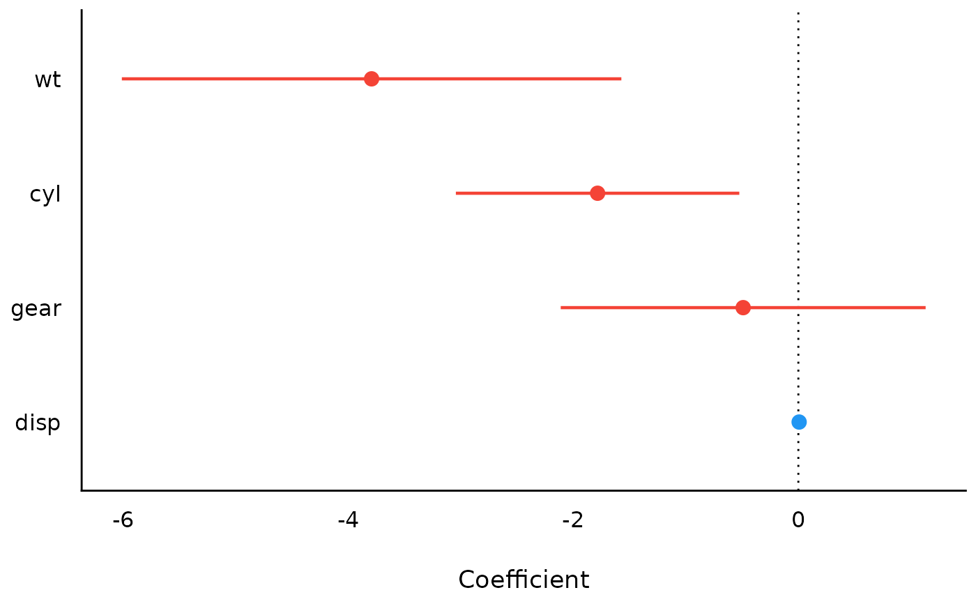
library(parameters)
m <- lm(mpg ~ wt + cyl + gear + disp, data = mtcars)
result <- model_parameters(m)
result
#> Parameter   | Coefficient |   SE |         95% CI | t(27) |      p
#> ------------------------------------------------------------------
#> (Intercept) |       43.54 | 4.86 | [33.57, 53.51] |  8.96 | < .001
#> wt          |       -3.79 | 1.08 | [-6.01, -1.57] | -3.51 | 0.002 
#> cyl         |       -1.78 | 0.61 | [-3.04, -0.52] | -2.91 | 0.007 
#> gear        |       -0.49 | 0.79 | [-2.11,  1.13] | -0.62 | 0.540 
#> disp        |    6.94e-03 | 0.01 | [-0.02,  0.03] |  0.58 | 0.568 
#> 
#> Uncertainty intervals (equal-tailed) and p-values (two-tailed) computed
#>   using a Wald t-distribution approximation.
plot(result)