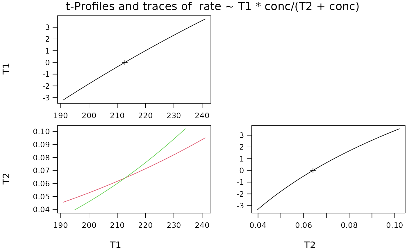
Plot a profile.nls Object With Profile Traces
p.profileTraces.RdDisplays a series of plots of the profile t function and the likelihood
profile traces for the parameters in a nonlinear regression model that
has been fitted with nls and profiled with
profile.nls.
Arguments
- x
an object of class
"profile.nls", typically resulting fromprofile(nls(.)), seeprofile.nls.- cex
character expansion, see
par(cex =).- subtitle
a subtitle to set for the plot. The default now includes the
nls()formula used.
Note
the stats-internal stats:::plot.profile.nls plot
method just does “the diagonals”.
Examples
require(stats)
data(Puromycin)
Treat <- Puromycin[Puromycin$state == "treated", ]
fm <- nls(rate ~ T1*conc/(T2+conc), data=Treat,
start = list(T1=207,T2=0.06))
(pr <- profile(fm)) # quite a few things..
#> $T1
#> tau par.vals.T1 par.vals.T2
#> 1 -3.209 190.8634 0.0455
#> 2 -2.563 195.0840 0.0488
#> 3 -1.916 199.3911 0.0523
#> 4 -1.269 203.7889 0.0560
#> 5 -0.621 208.2802 0.0600
#> 6 0.000 212.6837 0.0641
#> 7 0.609 217.0872 0.0684
#> 8 1.229 221.6741 0.0730
#> 9 1.848 226.3617 0.0780
#> 10 2.468 231.1568 0.0833
#> 11 3.086 236.0657 0.0890
#> 12 3.704 241.0959 0.0951
#>
#> $T2
#> tau par.vals.T1 par.vals.T2
#> 1 -3.356 195.0005 0.0397
#> 2 -2.672 198.4424 0.0440
#> 3 -1.988 201.9612 0.0486
#> 4 -1.305 205.5617 0.0535
#> 5 -0.624 209.2376 0.0589
#> 6 0.000 212.6837 0.0641
#> 7 0.583 215.9820 0.0694
#> 8 1.177 219.4187 0.0751
#> 9 1.770 222.9382 0.0812
#> 10 2.363 226.5483 0.0877
#> 11 2.955 230.2558 0.0946
#> 12 3.547 234.0683 0.1021
#>
#> attr(,"original.fit")
#> Nonlinear regression model
#> model: rate ~ T1 * conc/(T2 + conc)
#> data: Treat
#> T1 T2
#> 212.6837 0.0641
#> residual sum-of-squares: 1195
#>
#> Number of iterations to convergence: 5
#> Achieved convergence tolerance: 1.38e-06
#> attr(,"summary")
#>
#> Formula: rate ~ T1 * conc/(T2 + conc)
#>
#> Parameters:
#> Estimate Std. Error t value Pr(>|t|)
#> T1 2.13e+02 6.95e+00 30.61 3.2e-11 ***
#> T2 6.41e-02 8.28e-03 7.74 1.6e-05 ***
#> ---
#> Signif. codes: 0 ‘***’ 0.001 ‘**’ 0.01 ‘*’ 0.05 ‘.’ 0.1 ‘ ’ 1
#>
#> Residual standard error: 10.9 on 10 degrees of freedom
#>
#> Number of iterations to convergence: 5
#> Achieved convergence tolerance: 1.38e-06
#>
#> attr(,"class")
#> [1] "profile.nls" "profile"
op <- par(mfcol=1:2)
plot(pr) # -> 2 'standard' plots
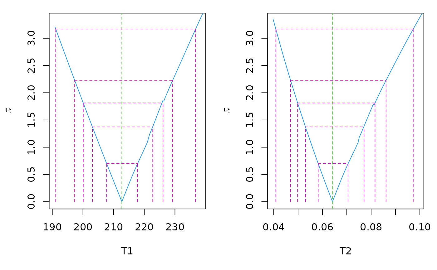 par(op)
## ours:
p.profileTraces(pr)
par(op)
## ours:
p.profileTraces(pr)