plot.ts with multi-plots and Auto-Title – on 1 page
p.ts.RdFor longer time-series, it is sometimes important to spread the time-series plots over several subplots. p.ts(.) does this both automatically, and under manual control.
Actually, this is a generalization of plot.ts
(with different defaults).
Arguments
- x
timeseries (possibly multivariate) or numeric vector.
- nrplots
number of sub-plots. Default: in {1..8}, approximately
n/400if possible.- overlap
by how much should subsequent plots overlap. Defaults to about 1/16 of sub-length on each side.
- date.x
a time “vector” of the same length as
xand coercable to class"POSIXct"(see DateTimeClasses).- do.x.axis
logical specifying if an x axis should be drawn (i.e., tick marks and labels).
- do.x.rug
logical specifying if
rugofdate.xvalues should drawn along the x axis.- ax.format
when
do.x.axisis true, specify theformatto be used in the call toaxis.POSIXct.- main.tit
Main title (over all plots). Defaults to name of
x.- ylim
numeric(2) or NULL; if the former, specifying the y-range for the plots. Defaults to a common pretty range.
- ylab, xlab
labels for y- and x-axis respectively, see description in
plot.default.- quiet
logical; if
TRUE, there's no reporting on each subplot.- mgp
- ...
further graphic parameters for each
plot.ts(..).
Side Effects
A page of nrplots subplots is drawn on the current
graphics device.
Examples
stopifnot(require(stats))
## stopifnot(require(datasets))
data(sunspots)
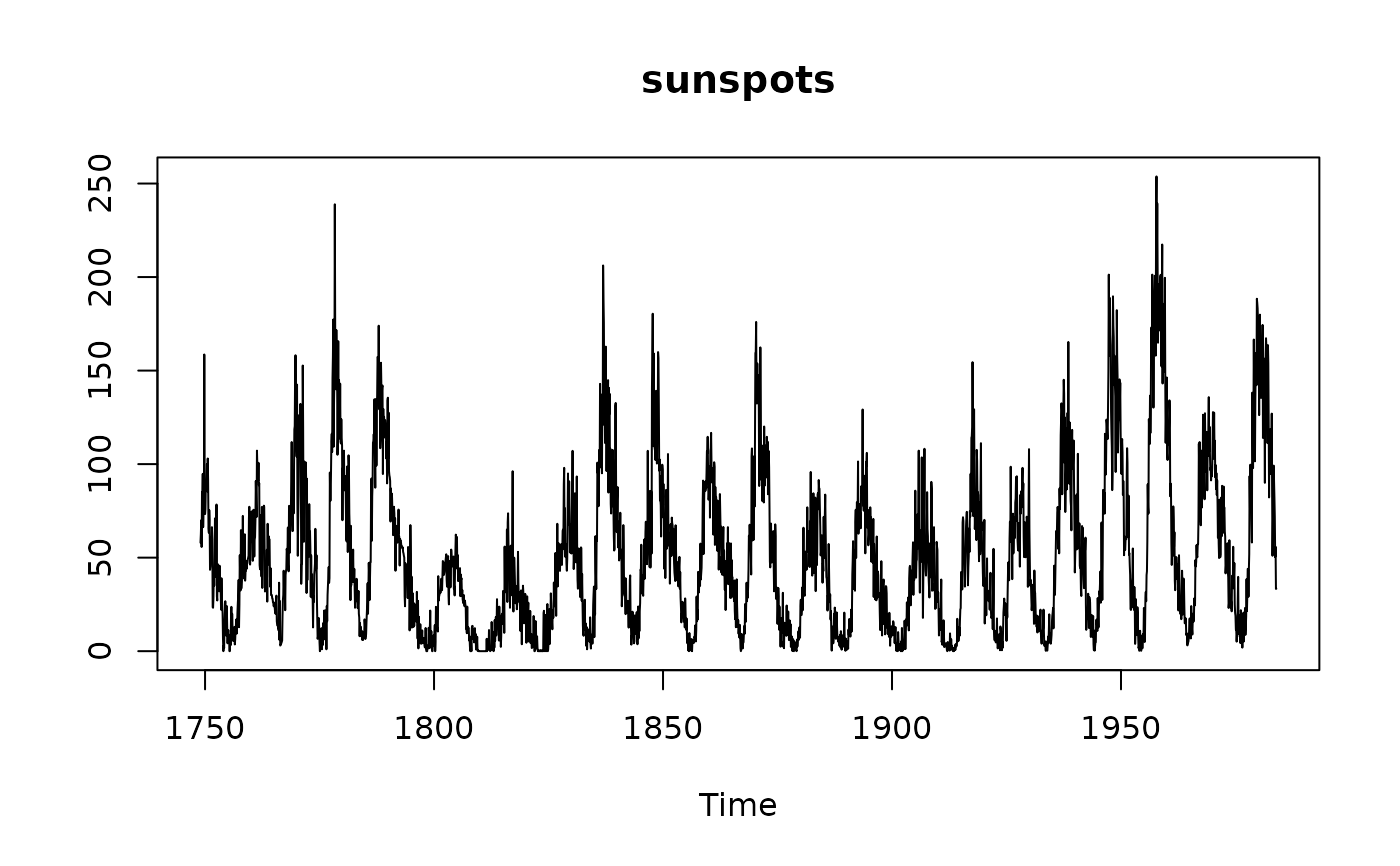
p.ts(sunspots, nr=1) # == usual plot.ts(..)
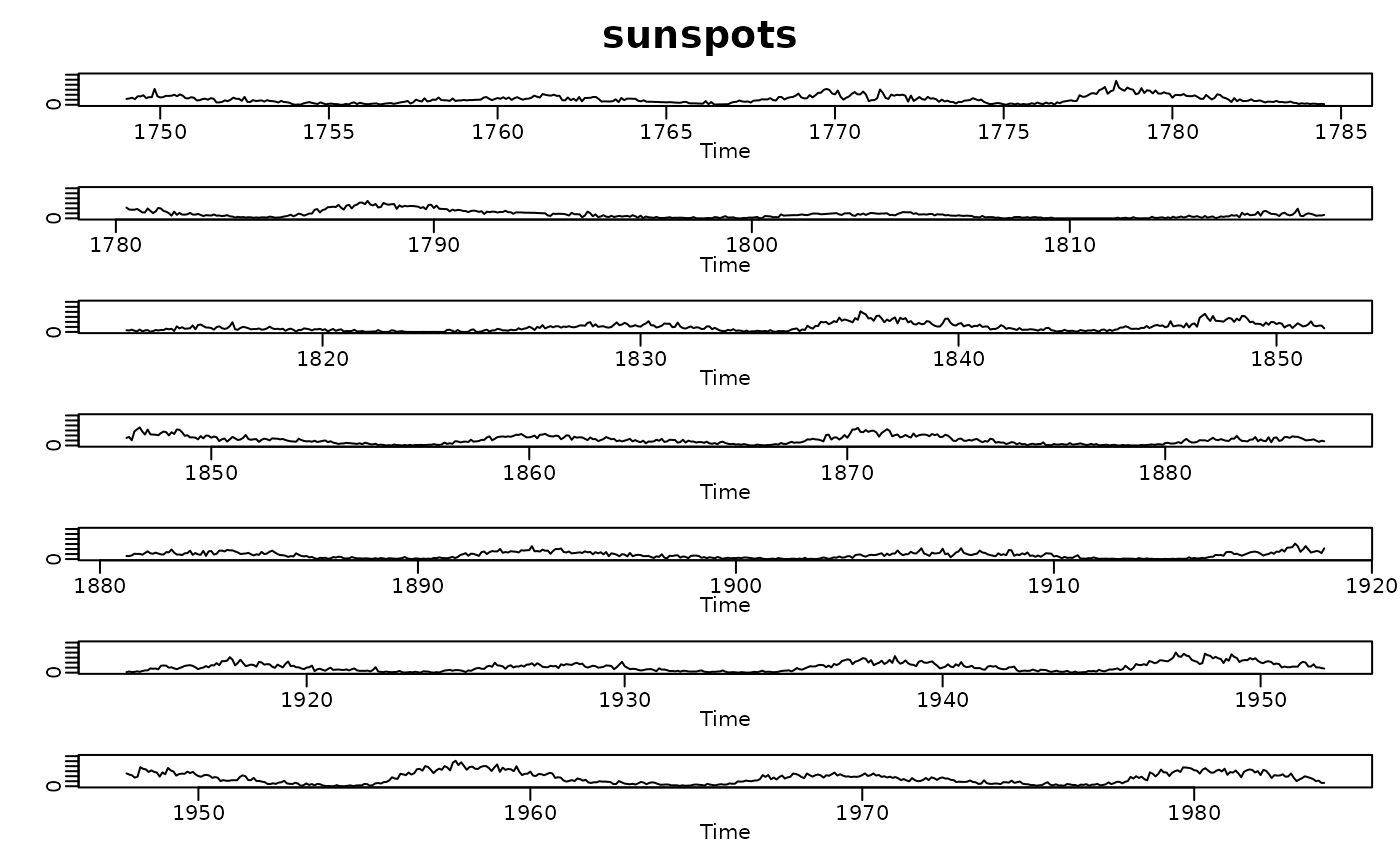
 p.ts(sunspots)
#> 1 -- start{0}= (1749, 1); end{426}= (1784.36, 2.66229)
#> 2 -- start{376}= (1780.21, 2.46719); end{828}= (1817.73, 4.23093)
#> 3 -- start{778}= (1813.58, 4.03583); end{1230}= (1851.1, 5.79957)
#> 4 -- start{1180}= (1846.95, 5.60447); end{1632}= (1884.47, 7.36822)
#> 5 -- start{1582}= (1880.32, 7.17311); end{2034}= (1917.84, 8.93686)
#> 6 -- start{1984}= (1913.69, 8.74175); end{2436}= (1951.21, 10.5055)
#> 7 -- start{2386}= (1947.06, 10.3104); end{2819}= (1983, 12)
p.ts(sunspots)
#> 1 -- start{0}= (1749, 1); end{426}= (1784.36, 2.66229)
#> 2 -- start{376}= (1780.21, 2.46719); end{828}= (1817.73, 4.23093)
#> 3 -- start{778}= (1813.58, 4.03583); end{1230}= (1851.1, 5.79957)
#> 4 -- start{1180}= (1846.95, 5.60447); end{1632}= (1884.47, 7.36822)
#> 5 -- start{1582}= (1880.32, 7.17311); end{2034}= (1917.84, 8.93686)
#> 6 -- start{1984}= (1913.69, 8.74175); end{2436}= (1951.21, 10.5055)
#> 7 -- start{2386}= (1947.06, 10.3104); end{2819}= (1983, 12)
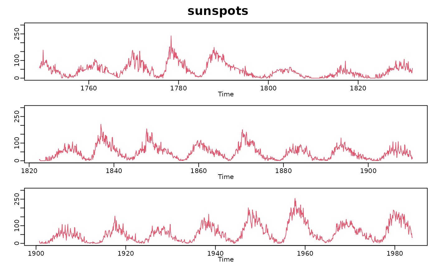
 p.ts(sunspots, nr=3, col=2)
#> 1 -- start{0}= (1749, 1); end{997}= (1831.76, 4.89039)
#> 2 -- start{881}= (1822.13, 4.43774); end{1937}= (1909.79, 8.55835)
#> 3 -- start{1821}= (1900.16, 8.10571); end{2819}= (1983, 12)
p.ts(sunspots, nr=3, col=2)
#> 1 -- start{0}= (1749, 1); end{997}= (1831.76, 4.89039)
#> 2 -- start{881}= (1822.13, 4.43774); end{1937}= (1909.79, 8.55835)
#> 3 -- start{1821}= (1900.16, 8.10571); end{2819}= (1983, 12)
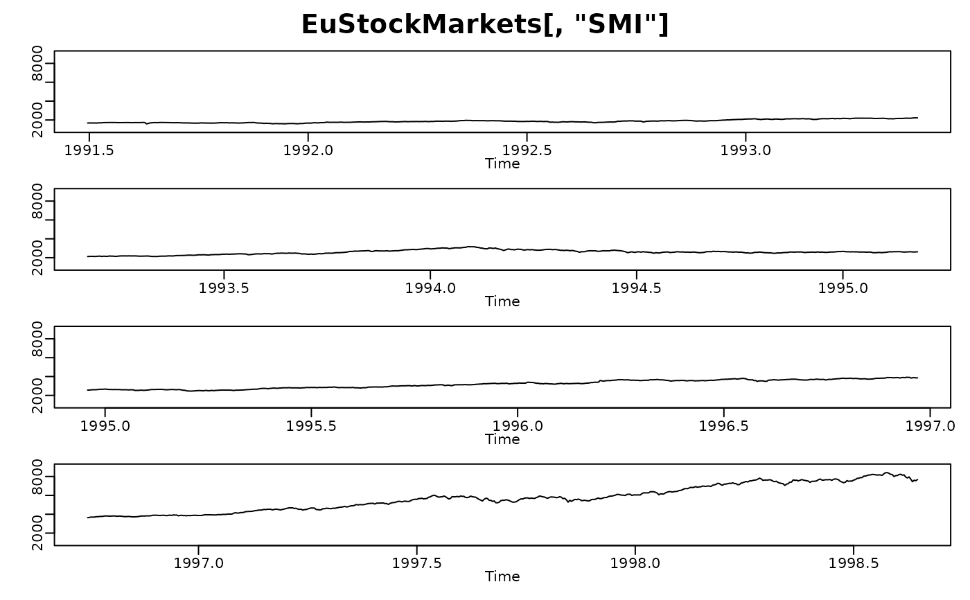
 data(EuStockMarkets)
p.ts(EuStockMarkets[,"SMI"])
#> 1 -- start{0}= (1991, 130); end{493}= (1992.86, 140.343)
#> 2 -- start{435}= (1992.64, 139.126); end{958}= (1994.61, 150.098)
#> 3 -- start{900}= (1994.39, 148.881); end{1423}= (1996.36, 159.853)
#> 4 -- start{1365}= (1996.14, 158.636); end{1859}= (1998, 169)
data(EuStockMarkets)
p.ts(EuStockMarkets[,"SMI"])
#> 1 -- start{0}= (1991, 130); end{493}= (1992.86, 140.343)
#> 2 -- start{435}= (1992.64, 139.126); end{958}= (1994.61, 150.098)
#> 3 -- start{900}= (1994.39, 148.881); end{1423}= (1996.36, 159.853)
#> 4 -- start{1365}= (1996.14, 158.636); end{1859}= (1998, 169)
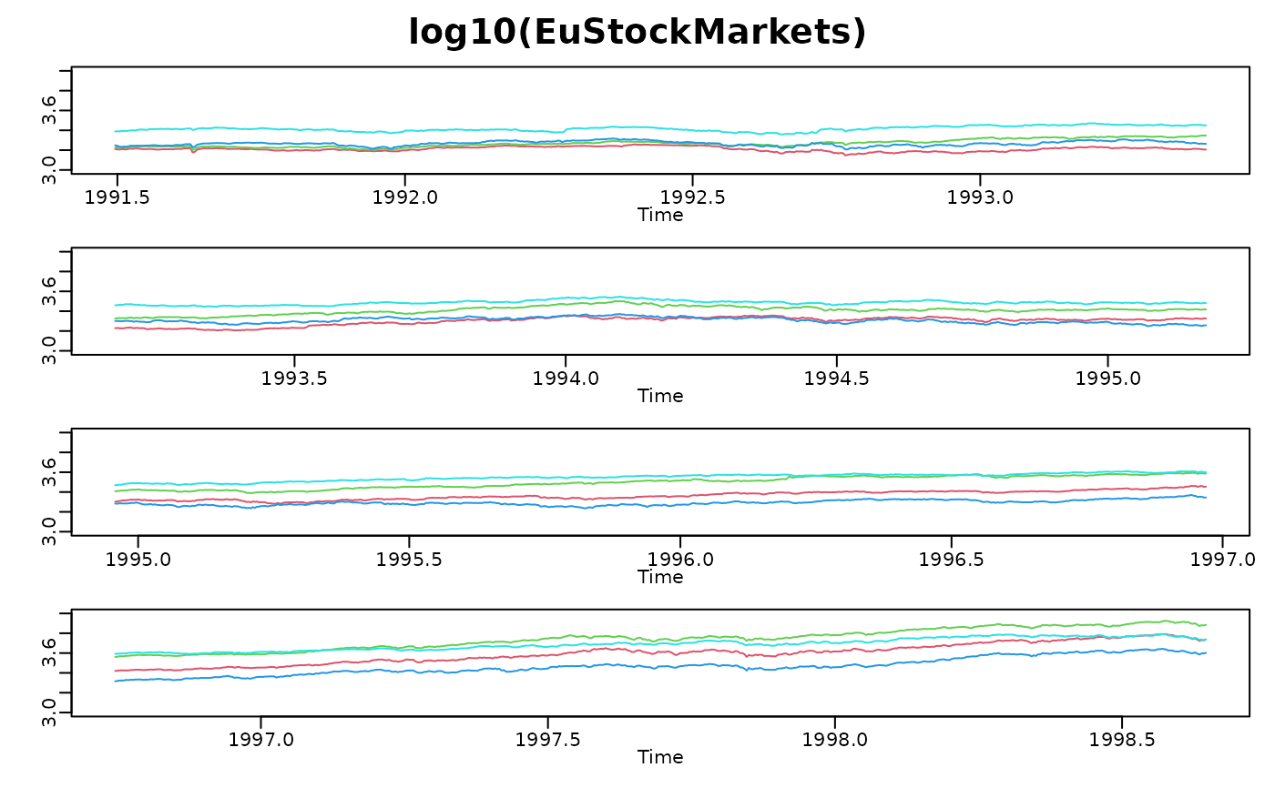
 ## multivariate :
p.ts(log10(EuStockMarkets), col = 2:5)
#> 1 -- start{0}= (1991, 130); end{493}= (1992.86, 140.343)
#> 2 -- start{435}= (1992.64, 139.126); end{958}= (1994.61, 150.098)
#> 3 -- start{900}= (1994.39, 148.881); end{1423}= (1996.36, 159.853)
#> 4 -- start{1365}= (1996.14, 158.636); end{1859}= (1998, 169)
## multivariate :
p.ts(log10(EuStockMarkets), col = 2:5)
#> 1 -- start{0}= (1991, 130); end{493}= (1992.86, 140.343)
#> 2 -- start{435}= (1992.64, 139.126); end{958}= (1994.61, 150.098)
#> 3 -- start{900}= (1994.39, 148.881); end{1423}= (1996.36, 159.853)
#> 4 -- start{1365}= (1996.14, 158.636); end{1859}= (1998, 169)
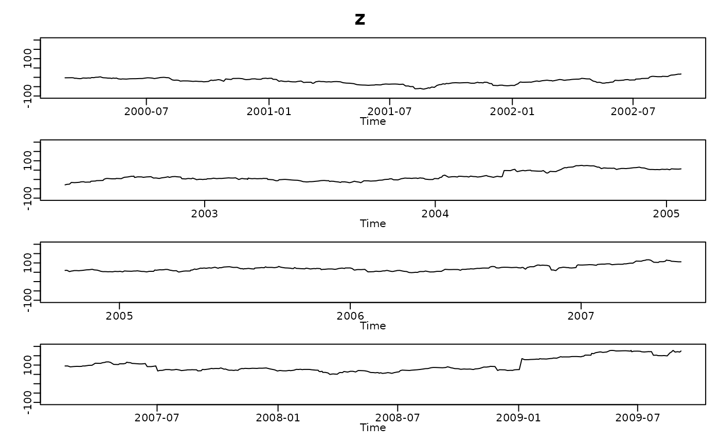
 ## with Date - x-axis (dense random dates):
set.seed(12)
x <- as.Date("2000-02-29") + cumsum(1+ rpois(1000, lambda= 2.5))
z <- cumsum(.1 + 2*rt(1000, df=3))
p.ts(z, 4, date.x = x)
#> 1 -- start{0}= (1, 1); end{264}= (265, 1)
#> summary(date.x):
#> Min. 1st Qu. Median
#> "2000-03-01 00:00:00.000" "2000-10-13 00:00:00.000" "2001-06-17 00:00:00.000"
#> Mean 3rd Qu. Max.
#> "2001-06-05 10:24:54.339" "2002-01-27 00:00:00.000" "2002-09-11 00:00:00.000"
#> 2 -- start{234}= (235, 1); end{514}= (515, 1)
#> summary(date.x):
#> Min. 1st Qu. Median
#> "2002-05-25 00:00:00.000" "2003-01-31 00:00:00.000" "2003-09-21 00:00:00.000"
#> Mean 3rd Qu. Max.
#> "2003-09-27 11:01:04.056" "2004-05-31 00:00:00.000" "2005-01-24 00:00:00.000"
#> 3 -- start{484}= (485, 1); end{764}= (765, 1)
#> summary(date.x):
#> Min. 1st Qu. Median
#> "2004-10-07 00:00:00.000" "2005-06-11 00:00:00.000" "2006-01-29 00:00:00.000"
#> Mean 3rd Qu. Max.
#> "2006-02-01 18:06:24.341" "2006-10-05 00:00:00.000" "2007-06-08 00:00:00.000"
#> 4 -- start{734}= (735, 1); end{999}= (1000, 1)
## with Date - x-axis (dense random dates):
set.seed(12)
x <- as.Date("2000-02-29") + cumsum(1+ rpois(1000, lambda= 2.5))
z <- cumsum(.1 + 2*rt(1000, df=3))
p.ts(z, 4, date.x = x)
#> 1 -- start{0}= (1, 1); end{264}= (265, 1)
#> summary(date.x):
#> Min. 1st Qu. Median
#> "2000-03-01 00:00:00.000" "2000-10-13 00:00:00.000" "2001-06-17 00:00:00.000"
#> Mean 3rd Qu. Max.
#> "2001-06-05 10:24:54.339" "2002-01-27 00:00:00.000" "2002-09-11 00:00:00.000"
#> 2 -- start{234}= (235, 1); end{514}= (515, 1)
#> summary(date.x):
#> Min. 1st Qu. Median
#> "2002-05-25 00:00:00.000" "2003-01-31 00:00:00.000" "2003-09-21 00:00:00.000"
#> Mean 3rd Qu. Max.
#> "2003-09-27 11:01:04.056" "2004-05-31 00:00:00.000" "2005-01-24 00:00:00.000"
#> 3 -- start{484}= (485, 1); end{764}= (765, 1)
#> summary(date.x):
#> Min. 1st Qu. Median
#> "2004-10-07 00:00:00.000" "2005-06-11 00:00:00.000" "2006-01-29 00:00:00.000"
#> Mean 3rd Qu. Max.
#> "2006-02-01 18:06:24.341" "2006-10-05 00:00:00.000" "2007-06-08 00:00:00.000"
#> 4 -- start{734}= (735, 1); end{999}= (1000, 1)
 #> summary(date.x):
#> Min. 1st Qu. Median
#> "2007-02-11 00:00:00.000" "2007-10-07 06:00:00.000" "2008-05-18 12:00:00.000"
#> Mean 3rd Qu. Max.
#> "2008-05-23 21:50:04.511" "2009-01-05 00:00:00.000" "2009-09-05 00:00:00.000"
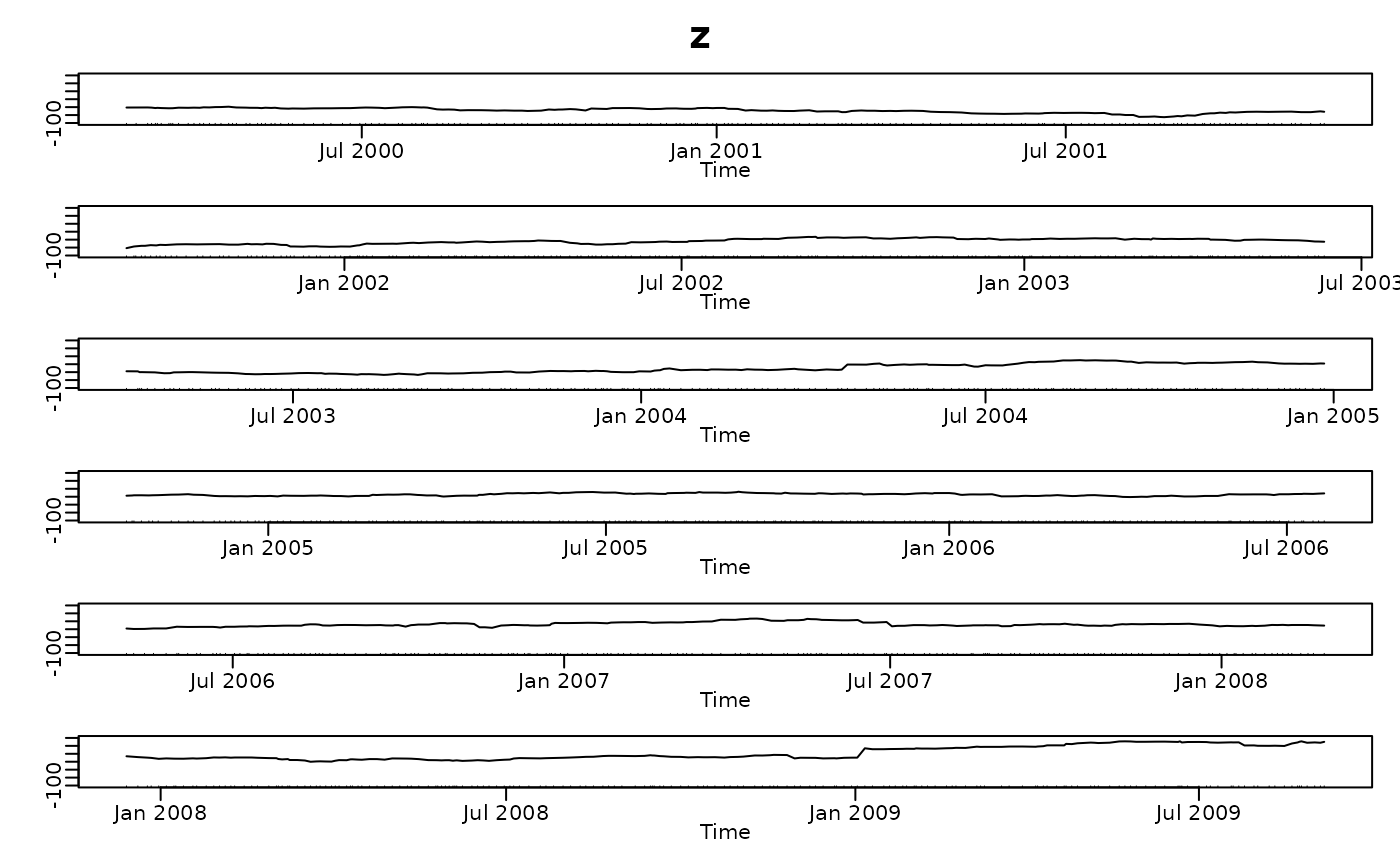
p.ts(z, 6, date.x = x, ax.format = "%b %Y", do.x.rug = TRUE)
#> 1 -- start{0}= (1, 1); end{175}= (176, 1)
#> summary(date.x):
#> Min. 1st Qu. Median
#> "2000-03-01 00:00:00.000" "2000-07-25 18:00:00.000" "2000-12-28 12:00:00.000"
#> Mean 3rd Qu. Max.
#> "2000-12-30 08:51:49.090" "2001-06-11 18:00:00.000" "2001-11-12 00:00:00.000"
#> 2 -- start{155}= (156, 1); end{341}= (342, 1)
#> summary(date.x):
#> Min. 1st Qu. Median
#> "2001-09-06 00:00:00.000" "2002-02-08 12:00:00.000" "2002-07-14 00:00:00.000"
#> Mean 3rd Qu. Max.
#> "2002-07-20 08:05:08.021" "2002-12-28 00:00:00.000" "2003-06-11 00:00:00.000"
#> 3 -- start{321}= (322, 1); end{507}= (508, 1)
#> summary(date.x):
#> Min. 1st Qu. Median
#> "2003-04-04 00:00:00.000" "2003-08-28 12:00:00.000" "2004-02-07 00:00:00.000"
#> Mean 3rd Qu. Max.
#> "2004-02-12 05:08:01.283" "2004-07-22 12:00:00.000" "2004-12-27 00:00:00.000"
#> 4 -- start{487}= (488, 1); end{673}= (674, 1)
#> summary(date.x):
#> Min. 1st Qu. Median
#> "2004-10-17 00:00:00.000" "2005-04-02 12:00:00.000" "2005-09-06 00:00:00.000"
#> Mean 3rd Qu. Max.
#> "2005-09-02 18:44:16.684" "2006-02-08 00:00:00.000" "2006-07-21 00:00:00.000"
#> 5 -- start{653}= (654, 1); end{839}= (840, 1)
#> summary(date.x):
#> Min. 1st Qu. Median
#> "2006-05-03 00:00:00.000" "2006-10-22 12:00:00.000" "2007-04-06 00:00:00.000"
#> Mean 3rd Qu. Max.
#> "2007-04-01 20:47:29.197" "2007-09-14 00:00:00.000" "2008-02-27 00:00:00.000"
#> 6 -- start{819}= (820, 1); end{999}= (1000, 1)
#> summary(date.x):
#> Min. 1st Qu. Median
#> "2007-02-11 00:00:00.000" "2007-10-07 06:00:00.000" "2008-05-18 12:00:00.000"
#> Mean 3rd Qu. Max.
#> "2008-05-23 21:50:04.511" "2009-01-05 00:00:00.000" "2009-09-05 00:00:00.000"
p.ts(z, 6, date.x = x, ax.format = "%b %Y", do.x.rug = TRUE)
#> 1 -- start{0}= (1, 1); end{175}= (176, 1)
#> summary(date.x):
#> Min. 1st Qu. Median
#> "2000-03-01 00:00:00.000" "2000-07-25 18:00:00.000" "2000-12-28 12:00:00.000"
#> Mean 3rd Qu. Max.
#> "2000-12-30 08:51:49.090" "2001-06-11 18:00:00.000" "2001-11-12 00:00:00.000"
#> 2 -- start{155}= (156, 1); end{341}= (342, 1)
#> summary(date.x):
#> Min. 1st Qu. Median
#> "2001-09-06 00:00:00.000" "2002-02-08 12:00:00.000" "2002-07-14 00:00:00.000"
#> Mean 3rd Qu. Max.
#> "2002-07-20 08:05:08.021" "2002-12-28 00:00:00.000" "2003-06-11 00:00:00.000"
#> 3 -- start{321}= (322, 1); end{507}= (508, 1)
#> summary(date.x):
#> Min. 1st Qu. Median
#> "2003-04-04 00:00:00.000" "2003-08-28 12:00:00.000" "2004-02-07 00:00:00.000"
#> Mean 3rd Qu. Max.
#> "2004-02-12 05:08:01.283" "2004-07-22 12:00:00.000" "2004-12-27 00:00:00.000"
#> 4 -- start{487}= (488, 1); end{673}= (674, 1)
#> summary(date.x):
#> Min. 1st Qu. Median
#> "2004-10-17 00:00:00.000" "2005-04-02 12:00:00.000" "2005-09-06 00:00:00.000"
#> Mean 3rd Qu. Max.
#> "2005-09-02 18:44:16.684" "2006-02-08 00:00:00.000" "2006-07-21 00:00:00.000"
#> 5 -- start{653}= (654, 1); end{839}= (840, 1)
#> summary(date.x):
#> Min. 1st Qu. Median
#> "2006-05-03 00:00:00.000" "2006-10-22 12:00:00.000" "2007-04-06 00:00:00.000"
#> Mean 3rd Qu. Max.
#> "2007-04-01 20:47:29.197" "2007-09-14 00:00:00.000" "2008-02-27 00:00:00.000"
#> 6 -- start{819}= (820, 1); end{999}= (1000, 1)
 #> summary(date.x):
#> Min. 1st Qu. Median
#> "2007-12-14 00:00:00.000" "2008-05-10 00:00:00.000" "2008-10-10 00:00:00.000"
#> Mean 3rd Qu. Max.
#> "2008-10-17 11:56:01.325" "2009-03-30 00:00:00.000" "2009-09-05 00:00:00.000"
#> summary(date.x):
#> Min. 1st Qu. Median
#> "2007-12-14 00:00:00.000" "2008-05-10 00:00:00.000" "2008-10-10 00:00:00.000"
#> Mean 3rd Qu. Max.
#> "2008-10-17 11:56:01.325" "2009-03-30 00:00:00.000" "2009-09-05 00:00:00.000"