Sequence Covering the Range of X, including X

Produce a sequence of unique values (sorted increasingly), containing the initial set of values x. This can be useful for setting prediction e.g. ranges in nonparametric regression.

seqXtend(x, length., method = c("simple", "aim", "interpolate"),
        from = NULL, to = NULL)

Arguments

x: numeric vector.
length.: integer specifying approximately the desired length() of the result.
method: string specifying the method to be used. The default, "simple" uses seq(*, length.out = length.) where "aim" aims a bit better towards the desired final length, and "interpolate" interpolates evenly inside each interval \([x_i, x_{i+1}]\) in a way to make all the new intervalls of approximately the same length.
from, to: numbers to be passed to (the default method for) seq(), defaulting to the minimal and maximal x value, respectively.

Note

method = "interpolate" typically gives the best results. Calling roundfixS, it also need more computational resources than the other methods.

Value

numeric vector of increasing values, of approximate length length. (unless length. < length(unique(x)) in which case, the result is simply sort(unique(x))), containing the original values of x.

From, r <- seqXtend(x, *), the original values are at indices ix <- match(x,r), i.e., identical(x, r[ix]).

Author

Martin Maechler

Examples

a <- c(1,2,10,12)
seqXtend(a, 12)# --> simply 1:12
#>  [1]  1  2  3  4  5  6  7  8  9 10 11 12
seqXtend(a, 12, "interp")# ditto
#>  [1]  1  2  3  4  5  6  7  8  9 10 11 12
seqXtend(a, 12, "aim")# really worse
#>  [1]  1.00  2.00  2.22  3.44  4.67  5.89  7.11  8.33  9.56 10.00 10.78 12.00
stopifnot(all.equal(seqXtend(a, 12, "interp"), 1:12))

## for a "general" x, however, "aim" aims better than default
x <- c(1.2, 2.4, 4.6, 9.9)
length(print(seqXtend(x, 12)))        # 14
#>  [1] 1.20 1.99 2.40 2.78 3.57 4.36 4.60 5.15 5.95 6.74 7.53 8.32 9.11 9.90
#> [1] 14
length(print(seqXtend(x, 12, "aim"))) # 12
#>  [1] 1.20 2.17 2.40 3.13 4.10 4.60 5.07 6.03 7.00 7.97 8.93 9.90
#> [1] 12
length(print(seqXtend(x, 12, "int"))) # 12
#>  [1] 1.20 2.40 3.13 3.87 4.60 5.36 6.11 6.87 7.63 8.39 9.14 9.90
#> [1] 12

## "interpolate" is really nice:
xt <- seqXtend(x, 100, "interp")
plot(xt, main="seqXtend(*, 100, \"interpol\")")
points(match(x,xt), x, col = 2, pch = 20)

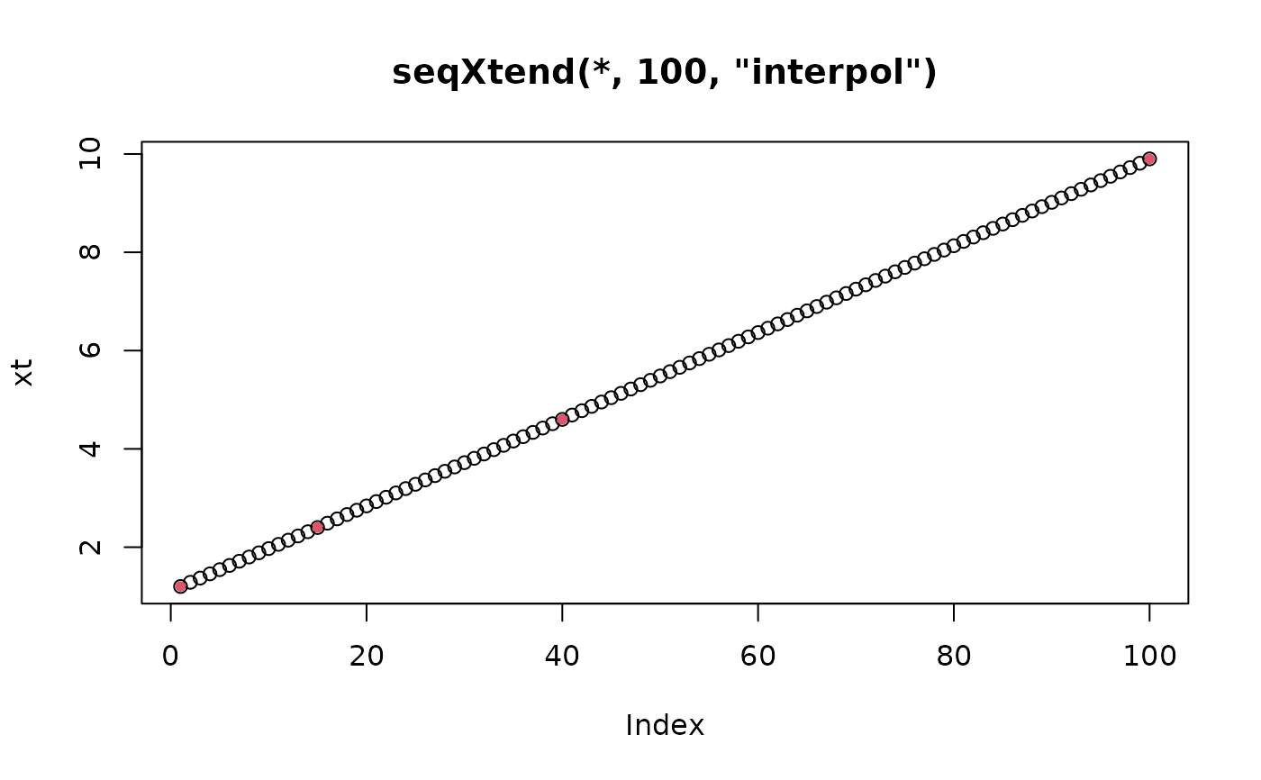# .... you don't even see that it's not equidistant
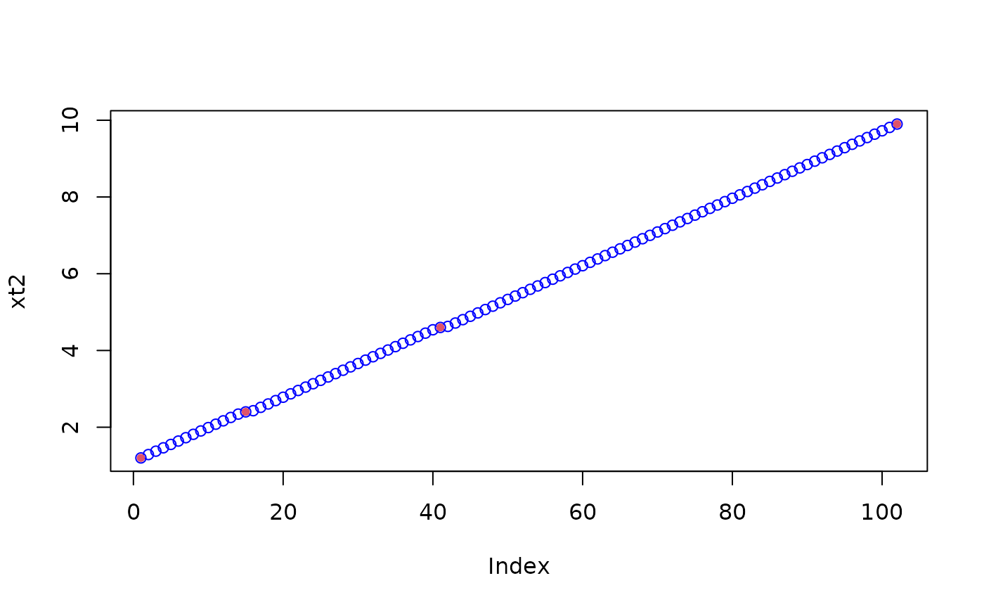
# whereas the cheap method shows ...
xt2 <- seqXtend(x, 100)
plot(xt2, col="blue")
points(match(x,xt2), x, col = 2, pch = 20)


## with "Date" objects
Drng <- as.Date(c("2007-11-10", "2012-07-12"))
(px <- pretty(Drng, n = 16)) # say, for the main labels
#>  [1] "2007-10-01" "2008-01-01" "2008-04-01" "2008-07-01" "2008-10-01"
#>  [6] "2009-01-01" "2009-04-01" "2009-07-01" "2009-10-01" "2010-01-01"
#> [11] "2010-04-01" "2010-07-01" "2010-10-01" "2011-01-01" "2011-04-01"
#> [16] "2011-07-01" "2011-10-01" "2012-01-01" "2012-04-01" "2012-07-01"
#> [21] "2012-10-01"
## say, a finer grid, for ticks -- should be almost equidistant
n3 <- 3*length(px)
summary(as.numeric(diff(seqXtend(px, n3))))        # wildly varying
#>    Min. 1st Qu.  Median    Mean 3rd Qu.    Max. 
#>     0.5    16.0    29.5    22.6    29.5    29.5 
summary(as.numeric(diff(seqXtend(px, n3, "aim")))) #   (ditto)
#>    Min. 1st Qu.  Median    Mean 3rd Qu.    Max. 
#>     1.7    17.1    33.8    29.5    42.5    42.5 
summary(as.numeric(diff(seqXtend(px, n3, "int")))) # around 30
#>    Min. 1st Qu.  Median    Mean 3rd Qu.    Max. 
#>    23.0    30.0    30.3    29.5    30.7    30.7