(Anti)Symmetric Log High-Transform
u.log.RdCompute \(log()\) only for high values and keep low ones –
antisymmetrically such that u.log(x) is (once) continuously
differentiable, it computes
\(f(x) = x\) for \(|x| \le c\) and
\(sign(x) c\cdot(1 + log(|x|/c))\)
for \(|x| \ge c\).
u.log(x, c = 1)Details
Alternatively, the ‘IHS’ (inverse hyperbolic sine)
transform has been proposed, first in more generality as \(S_U()\)
curves by Johnson(1949); in its simplest form,
\(f(x) = arsinh(x) = \log(x + \sqrt{x^2 + 1})\),
which is also antisymmetric, continous and once differentiable as our u.log(.).
See also
Value
numeric vector of same length as x.
References
N. L. Johnson (1949). Systems of Frequency Curves Generated by Methods of Translation, Biometrika 36, pp 149–176. doi:10.2307/2332539
Examples
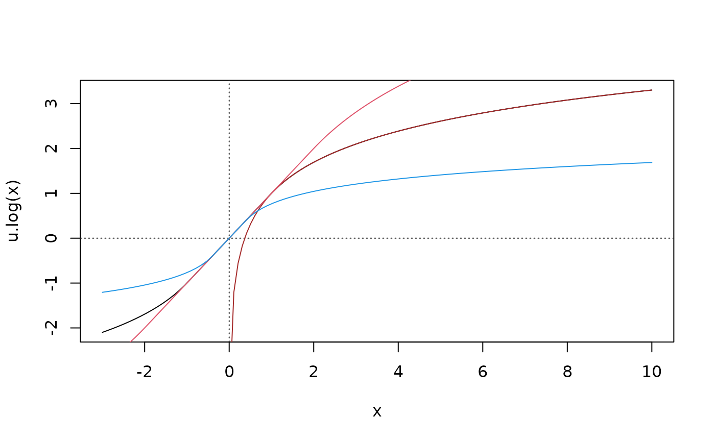
curve(u.log, -3, 10); abline(h=0, v=0, col = "gray20", lty = 3)
curve(1 + log(x), .01, add = TRUE, col= "brown") # simple log
curve(u.log(x, 2), add = TRUE, col=2)
curve(u.log(x, c= 0.4), add = TRUE, col=4)
 ## Compare with IHS = inverse hyperbolic sine == asinh
ihs <- function(x) log(x+sqrt(x^2+1)) # == asinh(x) {aka "arsinh(x)" or "sinh^{-1} (x)"}
xI <- c(-Inf, Inf, NA, NaN)
stopifnot(all.equal(xI, asinh(xI))) # but not for ihs():
cbind(xI, asinh=asinh(xI), ihs=ihs(xI)) # differs for -Inf
#> xI asinh ihs
#> [1,] -Inf -Inf NaN
#> [2,] Inf Inf Inf
#> [3,] NA NA NA
#> [4,] NaN NaN NaN
x <- runif(500, 0, 4); x[100+0:3] <- xI
all.equal(ihs(x), asinh(x)) #==> is.NA value mismatch: asinh() is correct {i.e. better!}
#> [1] "'is.NA' value mismatch: 2 in current 3 in target"
curve(u.log, -2, 20, n=1000); abline(h=0, v=0, col = "gray20", lty = 3)
curve(ihs(x)+1-log(2), add=TRUE, col=adjustcolor(2, 1/2), lwd=2)
curve(ihs(x), add=TRUE, col=adjustcolor(4, 1/2), lwd=2)
## Compare with IHS = inverse hyperbolic sine == asinh
ihs <- function(x) log(x+sqrt(x^2+1)) # == asinh(x) {aka "arsinh(x)" or "sinh^{-1} (x)"}
xI <- c(-Inf, Inf, NA, NaN)
stopifnot(all.equal(xI, asinh(xI))) # but not for ihs():
cbind(xI, asinh=asinh(xI), ihs=ihs(xI)) # differs for -Inf
#> xI asinh ihs
#> [1,] -Inf -Inf NaN
#> [2,] Inf Inf Inf
#> [3,] NA NA NA
#> [4,] NaN NaN NaN
x <- runif(500, 0, 4); x[100+0:3] <- xI
all.equal(ihs(x), asinh(x)) #==> is.NA value mismatch: asinh() is correct {i.e. better!}
#> [1] "'is.NA' value mismatch: 2 in current 3 in target"
curve(u.log, -2, 20, n=1000); abline(h=0, v=0, col = "gray20", lty = 3)
curve(ihs(x)+1-log(2), add=TRUE, col=adjustcolor(2, 1/2), lwd=2)
curve(ihs(x), add=TRUE, col=adjustcolor(4, 1/2), lwd=2)
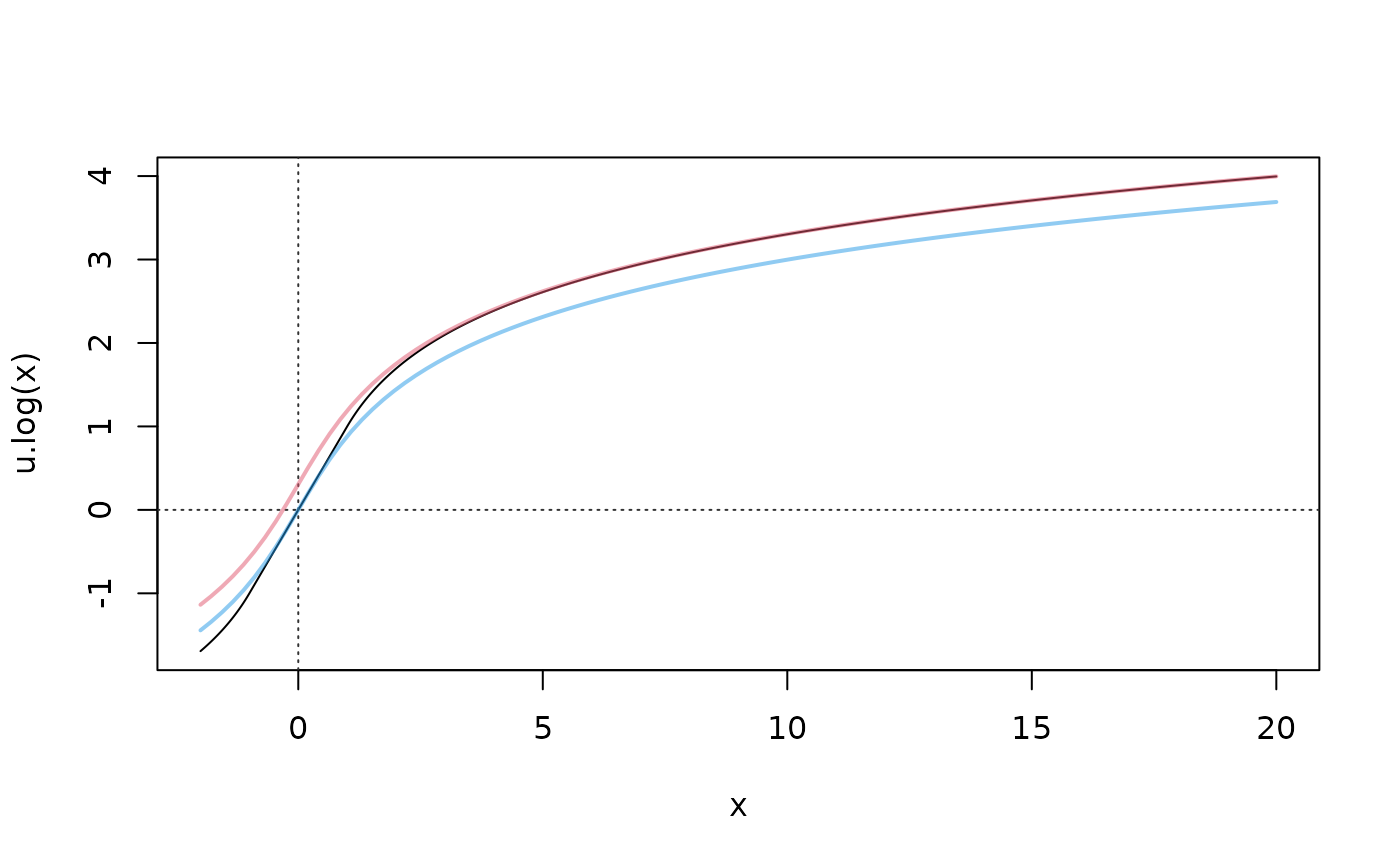 ## for x >= 0, u.log(x) is nicely between IHS(x) and shifted IHS
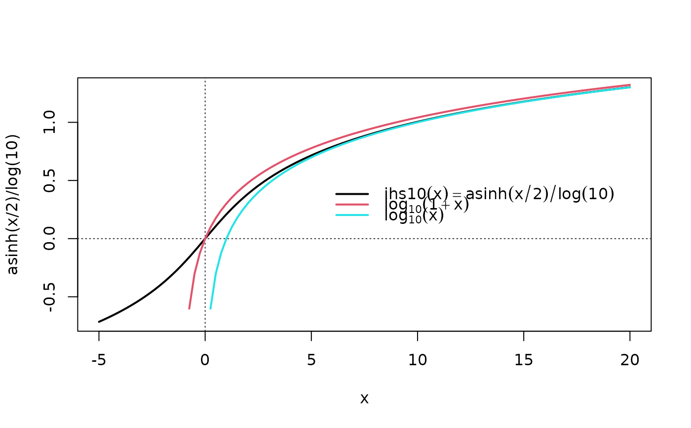
## a log10-scale version of asinh() {aka "IHS" }: ihs10(x) := asinh(x/2) / ln(10)
ihs10 <- function(x) asinh(x/2)/log(10)
xyaxis <- function() abline(h=0, v=0, col = "gray20", lty = 3)
leg3 <- function(x = "right")
legend(x, legend = c(quote(ihs10(x) == asinh(x/2)/log(10)),
quote(log[10](1+x)), quote(log[10](x))),
col=c(1,2,5), bty="n", lwd=2)
curve(asinh(x/2)/log(10), -5, 20, n=1000, lwd=2); xyaxis()
curve(log10(1+x), col=2, lwd=2, add=TRUE)
#> Warning: NaNs produced
curve(log10( x ), col=5, lwd=2, add=TRUE); leg3()
#> Warning: NaNs produced
## for x >= 0, u.log(x) is nicely between IHS(x) and shifted IHS
## a log10-scale version of asinh() {aka "IHS" }: ihs10(x) := asinh(x/2) / ln(10)
ihs10 <- function(x) asinh(x/2)/log(10)
xyaxis <- function() abline(h=0, v=0, col = "gray20", lty = 3)
leg3 <- function(x = "right")
legend(x, legend = c(quote(ihs10(x) == asinh(x/2)/log(10)),
quote(log[10](1+x)), quote(log[10](x))),
col=c(1,2,5), bty="n", lwd=2)
curve(asinh(x/2)/log(10), -5, 20, n=1000, lwd=2); xyaxis()
curve(log10(1+x), col=2, lwd=2, add=TRUE)
#> Warning: NaNs produced
curve(log10( x ), col=5, lwd=2, add=TRUE); leg3()
#> Warning: NaNs produced
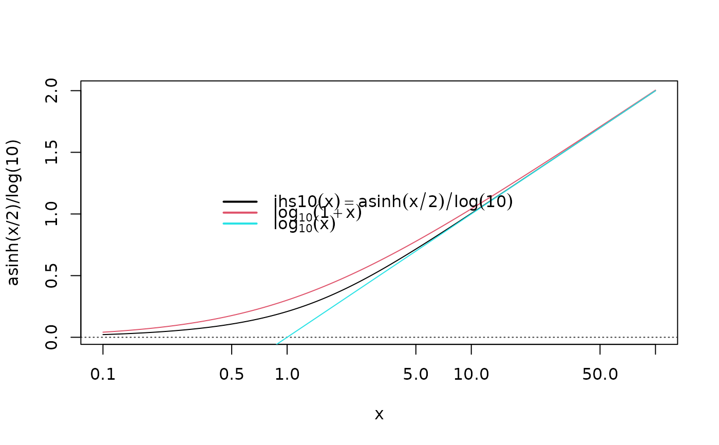
 ## zoom out and x-log-scale
curve(asinh(x/2)/log(10), .1, 100, log="x", n=1000); xyaxis()
curve(log10(1+x), col=2, add=TRUE)
curve(log10( x ), col=5, add=TRUE) ; leg3("center")
## zoom out and x-log-scale
curve(asinh(x/2)/log(10), .1, 100, log="x", n=1000); xyaxis()
curve(log10(1+x), col=2, add=TRUE)
curve(log10( x ), col=5, add=TRUE) ; leg3("center")
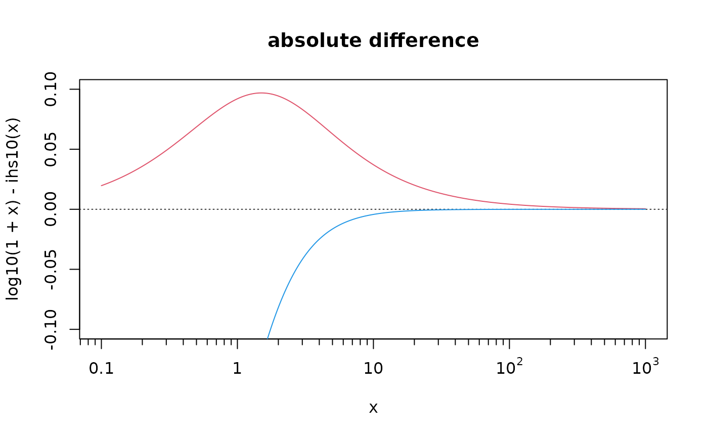
 curve(log10(1+x) - ihs10(x), .1, 1000, col=2, n=1000, log="x", ylim = c(-1,1)*0.10,
main = "absolute difference", xaxt="n"); xyaxis(); eaxis(1, sub10=1)
curve(log10( x ) - ihs10(x), col=4, n=1000, add = TRUE)
curve(log10(1+x) - ihs10(x), .1, 1000, col=2, n=1000, log="x", ylim = c(-1,1)*0.10,
main = "absolute difference", xaxt="n"); xyaxis(); eaxis(1, sub10=1)
curve(log10( x ) - ihs10(x), col=4, n=1000, add = TRUE)
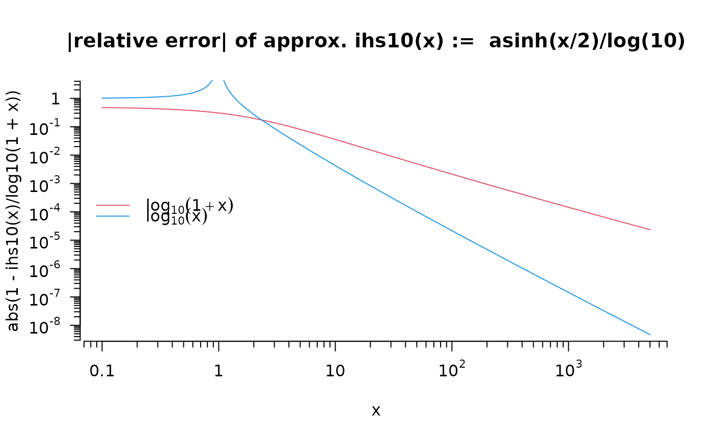
 curve(abs(1 - ihs10(x) / log10(1+x)), .1, 5000, col=2, log = "xy", ylim = c(6e-9, 2),
main="|relative error| of approx. ihs10(x) := asinh(x/2)/log(10)", n=1000, axes=FALSE)
eaxis(1, sub10=1); eaxis(2, sub10=TRUE)
curve(abs(1 - ihs10(x) / log10(x)), col=4, n=1000, add = TRUE)
legend("left", legend = c(quote(log[10](1+x)), quote(log[10](x))),
col=c(2,4), bty="n", lwd=1)
curve(abs(1 - ihs10(x) / log10(1+x)), .1, 5000, col=2, log = "xy", ylim = c(6e-9, 2),
main="|relative error| of approx. ihs10(x) := asinh(x/2)/log(10)", n=1000, axes=FALSE)
eaxis(1, sub10=1); eaxis(2, sub10=TRUE)
curve(abs(1 - ihs10(x) / log10(x)), col=4, n=1000, add = TRUE)
legend("left", legend = c(quote(log[10](1+x)), quote(log[10](x))),
col=c(2,4), bty="n", lwd=1)
 ## Compare with Stahel's version of "started log"
## (here, for *vectors* only, and 'base', as Desctools::LogSt();
## by MM: "modularized" by providing a threshold-computer function separately:
logst_thrWS <- function(x, mult = 1) {
lq <- quantile(x[x > 0], probs = c(0.25, 0.75), na.rm = TRUE, names = FALSE)
if (lq[1] == lq[2])
lq[1] <- lq[2]/2
lq[1]^(1 + mult)/lq[2]^mult
}
logst0L <- function(x, calib = x, threshold = thrFUN(calib, mult=mult),
thrFUN = logst_thrWS, mult = 1, base = 10)
{
## logical index sub-assignment instead of ifelse(): { already in DescTools::LogSt }
res <- x # incl NA's
notNA <- !is.na(sml <- (x < (th <- threshold)))
i1 <- sml & notNA; res[i1] <- log(th, base) + ((x[i1] - th)/(th * log(base)))
i2 <- !sml & notNA; res[i2] <- log(x[i2], base)
attr(res, "threshold") <- th
attr(res, "base") <- base
res
}
logst0 <- function(x, calib = x, threshold = thrFUN(calib, mult=mult),
thrFUN = logst_thrWS, mult = 1, base = 10)
{
## Using pmax.int() instead of logical indexing -- NA's work automatically - even faster
xm <- pmax.int(threshold, x)
res <- log(xm, base) + (x - xm)/(threshold * log(base))
attr(res, "threshold") <- threshold
attr(res, "base") <- base
res
}
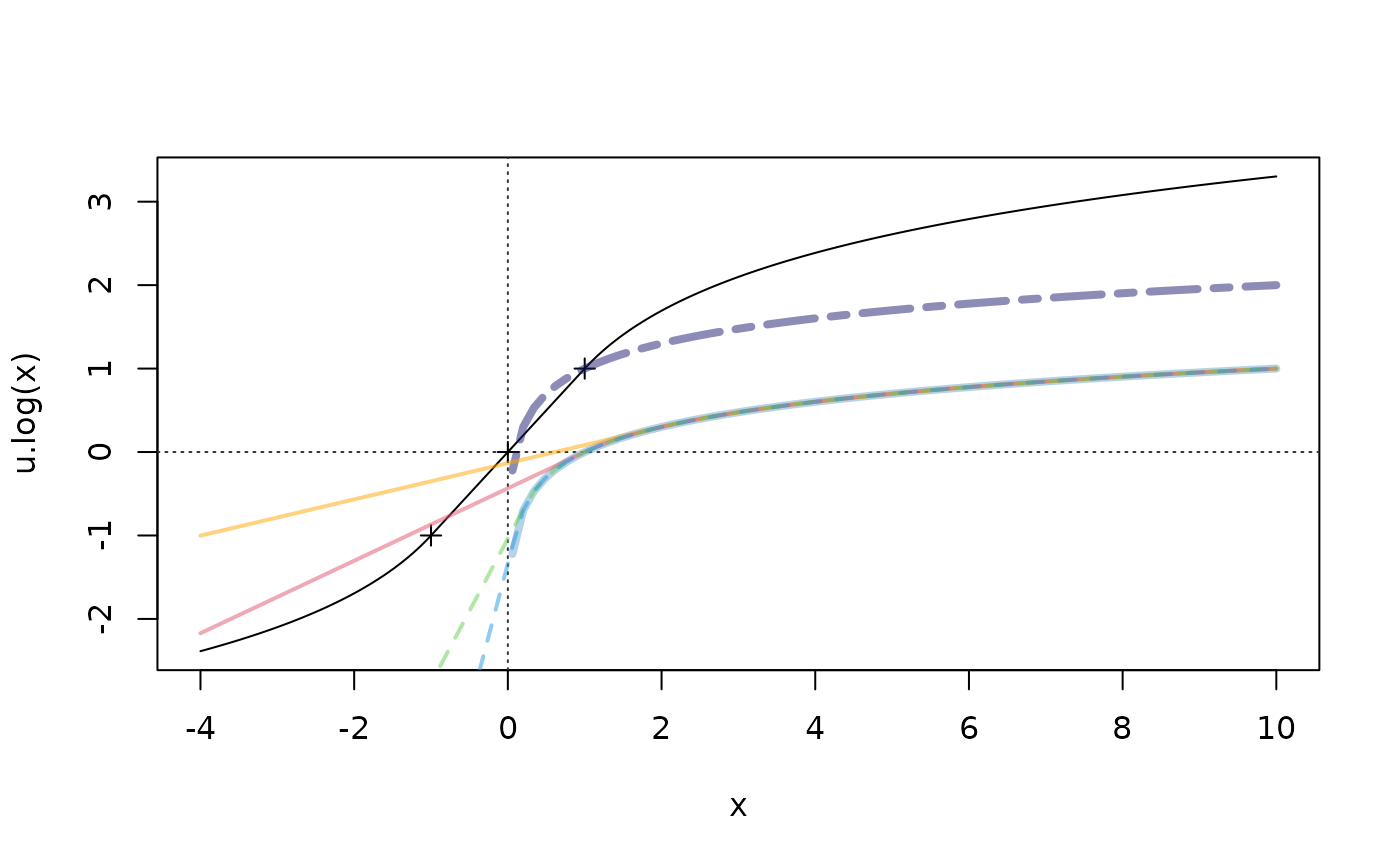
## u.log() is really using natural log() -- whereas logst() defaults to base=10
curve(u.log, -4, 10, n=1000); abline(h=0, v=0, col = "gray20", lty = 3); points(-1:1, -1:1, pch=3)
curve(log10(x) + 1, add=TRUE, col=adjustcolor("midnightblue", 1/2), lwd=4, lty=6)
#> Warning: NaNs produced
curve(log10(x), add=TRUE, col=adjustcolor("skyblue3", 1/2), lwd=4, lty=7)
#> Warning: NaNs produced
curve(logst0(x, threshold= 2 ), add=TRUE, col=adjustcolor("orange",1/2), lwd=2)
curve(logst0(x, threshold= 1 ), add=TRUE, col=adjustcolor(2, 1/2), lwd=2)
curve(logst0(x, threshold= 1/4), add=TRUE, col=adjustcolor(3, 1/2), lwd=2, lty=2)
curve(logst0(x, threshold= 1/8), add=TRUE, col=adjustcolor(4, 1/2), lwd=2, lty=2)
## Compare with Stahel's version of "started log"
## (here, for *vectors* only, and 'base', as Desctools::LogSt();
## by MM: "modularized" by providing a threshold-computer function separately:
logst_thrWS <- function(x, mult = 1) {
lq <- quantile(x[x > 0], probs = c(0.25, 0.75), na.rm = TRUE, names = FALSE)
if (lq[1] == lq[2])
lq[1] <- lq[2]/2
lq[1]^(1 + mult)/lq[2]^mult
}
logst0L <- function(x, calib = x, threshold = thrFUN(calib, mult=mult),
thrFUN = logst_thrWS, mult = 1, base = 10)
{
## logical index sub-assignment instead of ifelse(): { already in DescTools::LogSt }
res <- x # incl NA's
notNA <- !is.na(sml <- (x < (th <- threshold)))
i1 <- sml & notNA; res[i1] <- log(th, base) + ((x[i1] - th)/(th * log(base)))
i2 <- !sml & notNA; res[i2] <- log(x[i2], base)
attr(res, "threshold") <- th
attr(res, "base") <- base
res
}
logst0 <- function(x, calib = x, threshold = thrFUN(calib, mult=mult),
thrFUN = logst_thrWS, mult = 1, base = 10)
{
## Using pmax.int() instead of logical indexing -- NA's work automatically - even faster
xm <- pmax.int(threshold, x)
res <- log(xm, base) + (x - xm)/(threshold * log(base))
attr(res, "threshold") <- threshold
attr(res, "base") <- base
res
}
## u.log() is really using natural log() -- whereas logst() defaults to base=10
curve(u.log, -4, 10, n=1000); abline(h=0, v=0, col = "gray20", lty = 3); points(-1:1, -1:1, pch=3)
curve(log10(x) + 1, add=TRUE, col=adjustcolor("midnightblue", 1/2), lwd=4, lty=6)
#> Warning: NaNs produced
curve(log10(x), add=TRUE, col=adjustcolor("skyblue3", 1/2), lwd=4, lty=7)
#> Warning: NaNs produced
curve(logst0(x, threshold= 2 ), add=TRUE, col=adjustcolor("orange",1/2), lwd=2)
curve(logst0(x, threshold= 1 ), add=TRUE, col=adjustcolor(2, 1/2), lwd=2)
curve(logst0(x, threshold= 1/4), add=TRUE, col=adjustcolor(3, 1/2), lwd=2, lty=2)
curve(logst0(x, threshold= 1/8), add=TRUE, col=adjustcolor(4, 1/2), lwd=2, lty=2)