Plot Components + Residuals for Two Factors

For an analysis of variance or regression with (at least) two factors: Plot components + residuals for two factors according to Tukey's “forget-it plot”. Try it!

Usage

compresid2way(aov, data=NULL, fac=1:2, label = TRUE, numlabel = FALSE,
             xlab=NULL, ylab=NULL, main=NULL,
             col=c(2,3,4,4), lty=c(1,1,2,4), pch=c(1,2))

Arguments

aov: either an aov object with a formula of the form y ~ a + b, where a and b are factors, or such a formula.
data: data frame containing a and b.
fac: the two factors used for plotting. Either column numbers or names for argument data.
label: logical indicating if levels of factors should be shown in the plot.
numlabel: logical indicating if effects of factors will be shown in the plot.
xlab,ylab,main: the usual title components, here with a non-trivial default constructed from aov and the component factors used.
col,lty,pch: colors, line types, plotting characters to be used for plotting [1] positive residuals, [2] negative residuals, [3] grid, [4] labels. If pch is sufficiently long, it will be used as the list of individual symbols for plotting the y values.

Details

For a two-way analysis of variance, the plot shows the additive components of the fits for the two factors by the intersections of a grid, along with the residuals. The observed values of the target variable are identical to the vertical coordinate.

The application of the function has been extended to cover more complicated models. The components of the fit for two factors are shown as just described, and the residuals are added. The result is a “component plus residual” plot for two factors in one display.

Value

Invisibly, a list with components

compy: data.frame containing the component effects of the two factors, and combined effects plus residual
coef: coefficients: Intercept and effects of the factors

References

F. Mosteller and J. W. Tukey (1977) Data Analysis and Regression: A Second Course in Statistics. Addison-Wesley, Reading, Mass., p. 176.

John W. Tukey (1977) Exploratory Data Analysis. Addison-Wesley, Reading, Mass., p. 381.

Author

Werner Stahel stahel@stat.math.ethz.ch

Examples

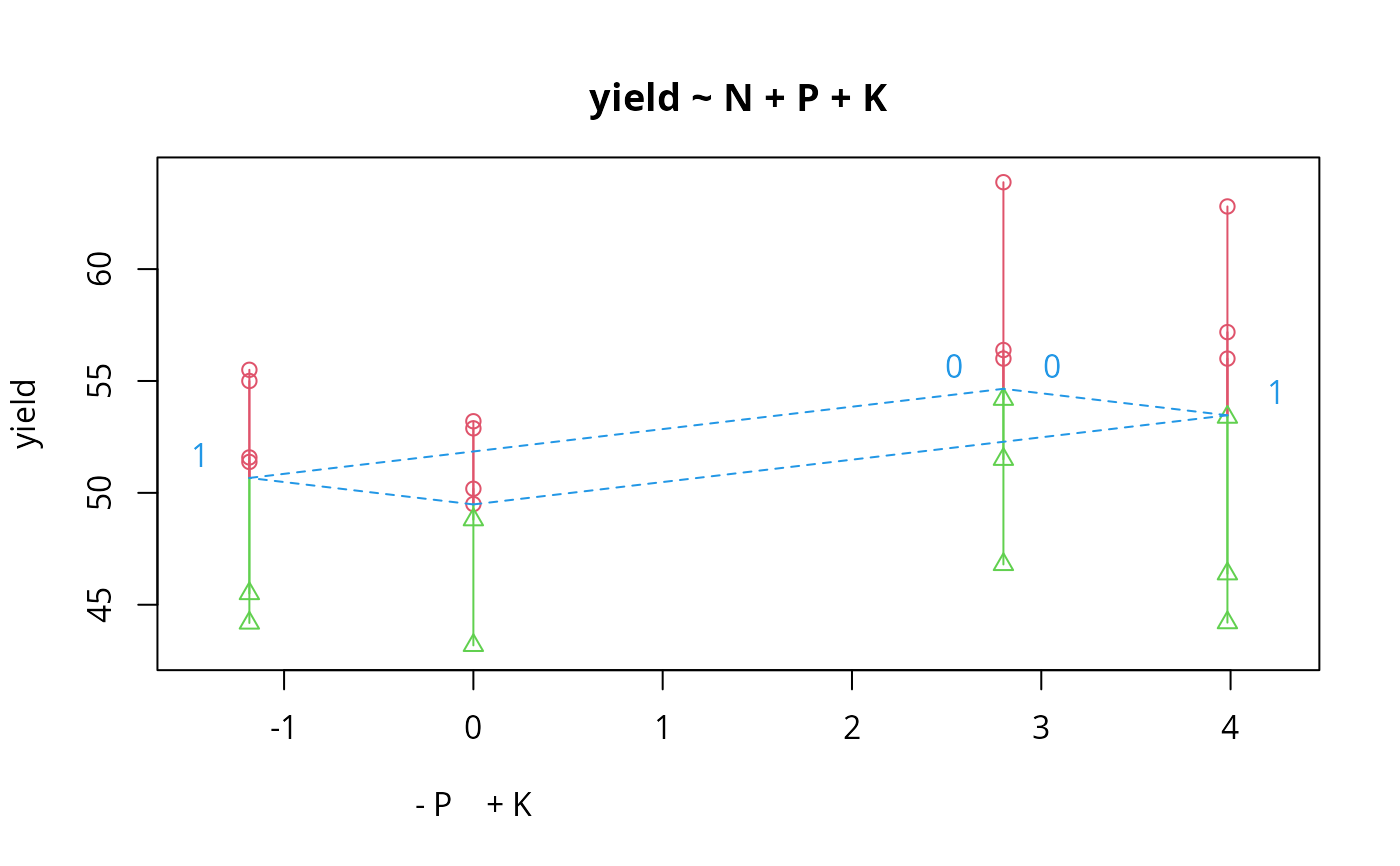
 ## From Venables and Ripley (2002) p.165.
 N <- c(0,1,0,1,1,1,0,0,0,1,1,0,1,1,0,0,1,0,1,0,1,1,0,0)
 P <- c(1,1,0,0,0,1,0,1,1,1,0,0,0,1,0,1,1,0,0,1,0,1,1,0)
 K <- c(1,0,0,1,0,1,1,0,0,1,0,1,0,1,1,0,0,0,1,1,1,0,1,0)
 yield <- c(49.5,62.8,46.8,57.0,59.8,58.5,55.5,56.0,62.8,55.8,69.5,55.0,
            62.0,48.8,45.5,44.2,52.0,51.5,49.8,48.8,57.2,59.0,53.2,56.0)
 npk <- data.frame(block=gl(6,4), N=factor(N), P=factor(P),
                   K=factor(K), yield=yield)
 npk.cr <- compresid2way(yield ~ N+P+K, data=npk, fac=c("P","K"))


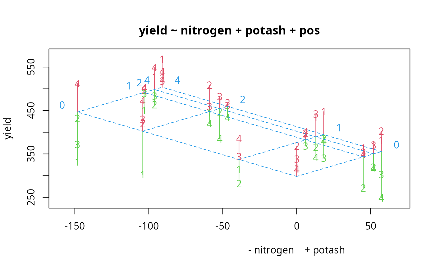
 ## Fisher's 1926 data on potatoe yield
 data(potatoes)
 pot.aov <- aov(yield ~ nitrogen+potash+pos, data=potatoes)
 compresid2way(pot.aov, pch=as.character(potatoes$pos))


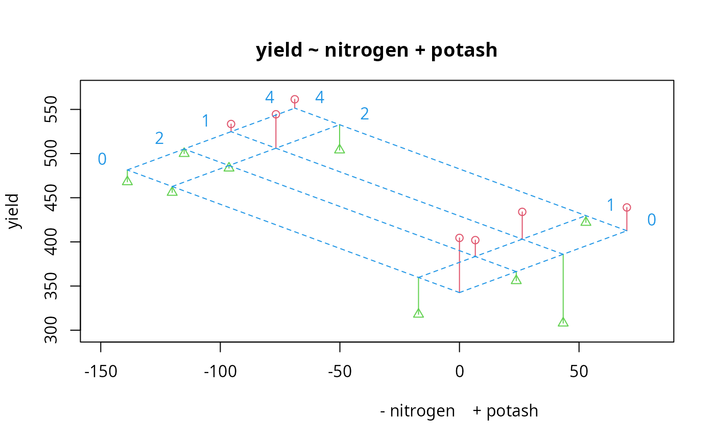
 compresid2way(yield~nitrogen+potash, data=subset(potatoes, pos == 2))


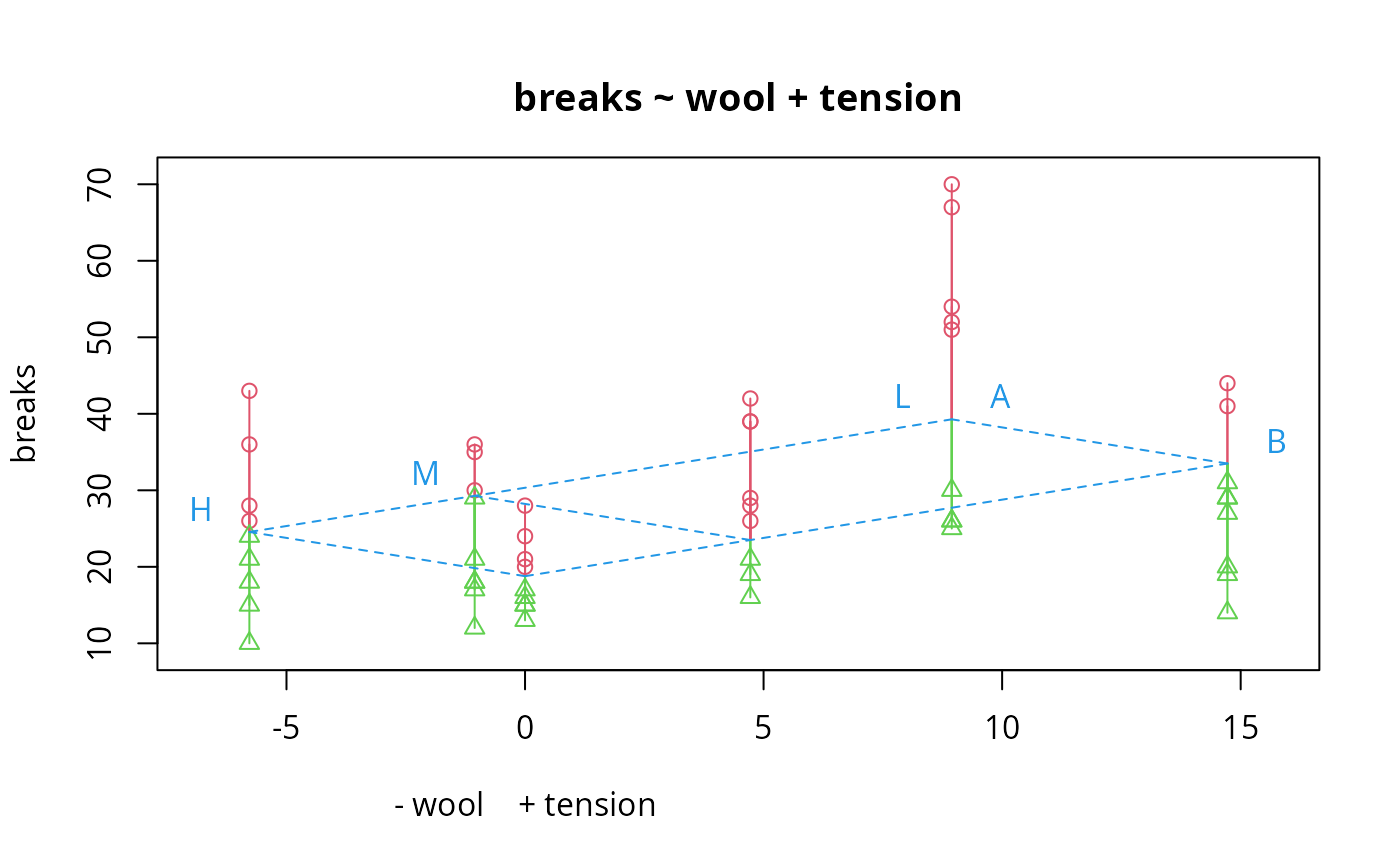
 ## 2 x 3 design :
 data(warpbreaks)
 summary(fm1 <- aov(breaks ~ wool + tension, data = warpbreaks))
#>             Df Sum Sq Mean Sq F value  Pr(>F)   
#> wool         1    451   450.7   3.339 0.07361 . 
#> tension      2   2034  1017.1   7.537 0.00138 **
#> Residuals   50   6748   135.0                   
#> ---
#> Signif. codes:  0 ‘***’ 0.001 ‘**’ 0.01 ‘*’ 0.05 ‘.’ 0.1 ‘ ’ 1
 compresid2way(fm1)