Plot Data and Smoother / Fitted Values

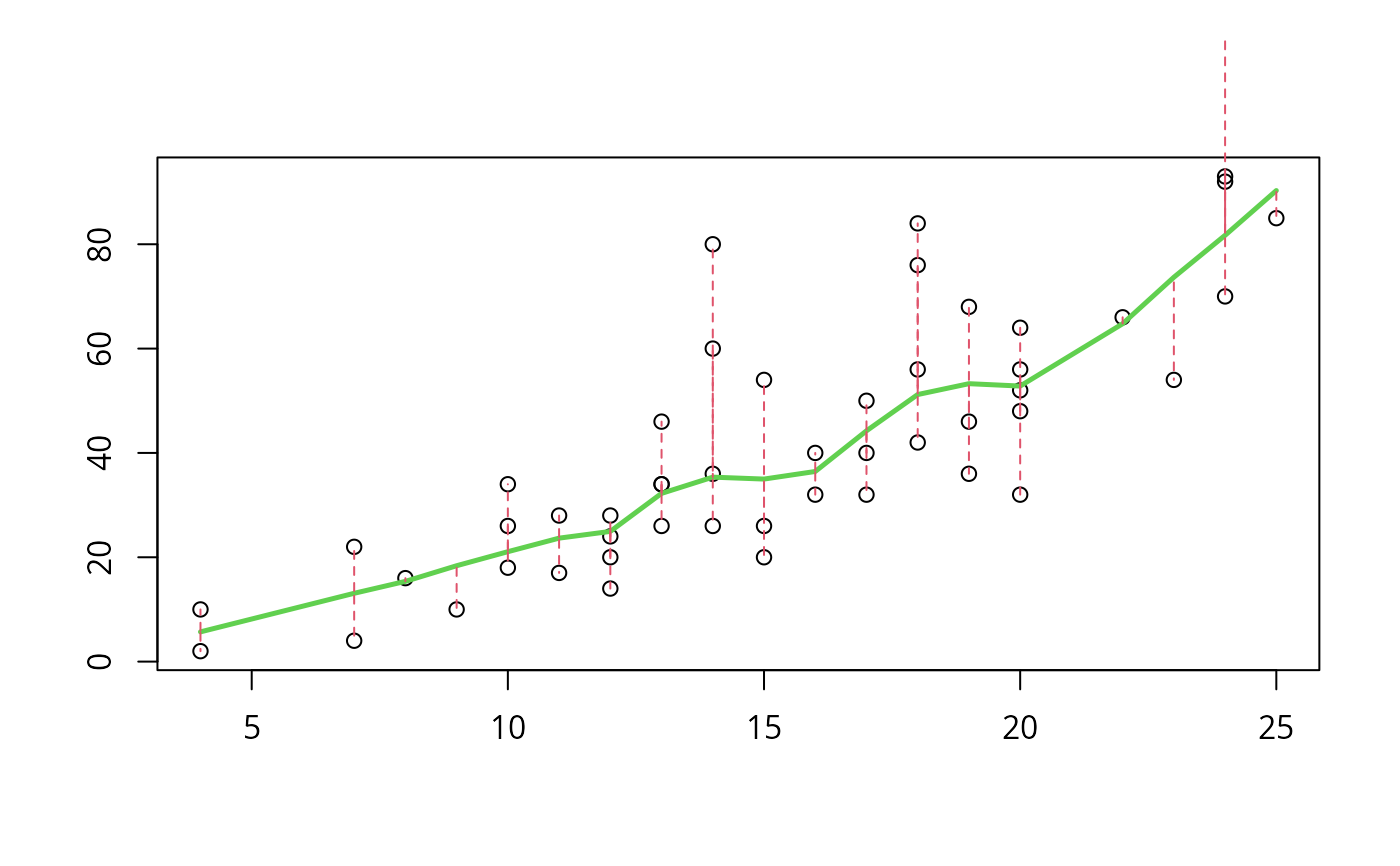
For one-dimensional nonparametric regression, plot the data and fitted values, typically a smooth function, and optionally use segments to visualize the residuals.

Usage

plotDS(x, yd, ys, xlab = "", ylab = "", ylim = rrange(c(yd, ys)),
       xpd = TRUE, do.seg = TRUE, seg.p = 0.95,
       segP = list(lty = 2, lwd = 1,   col = 2),
       linP = list(lty = 1, lwd = 2.5, col = 3),
       ...)

Arguments

x, yd, ys

numeric vectors all of the same length, representing \((x_i, y_i)\) and fitted (smooth) values \(\hat{y}_i\). x will be sorted increasingly if necessary, and yd and ys accordingly.

Alternatively, ys can be an x-y list (as resulting from xy.coords) containing fitted values on a finer grid than the observations x. In that case, the observational values x[] must be part of the larger set; seqXtend() may be applied to construct such a set of abscissa values.

xlab, ylab

x- and y- axis labels, as in plot.default.

ylim

limits of y-axis to be used; defaults to a robust range of the values.

xpd

see par(xpd=.); by default do allow to draw outside the plot region.

do.seg

logical indicating if residual segments should be drawn, at x[i], from yd[i] to ys[i] (approximately, see seg.p).

seg.p

segment percentage of segments to be drawn, from yd to seg.p*ys + (1-seg.p)*yd.

segP

list with named components lty, lwd, col specifying line type, width and color for the residual segments, used only when do.seg is true.

linP

list with named components lty, lwd, col specifying line type, width and color for “smooth curve lines”.

...

further arguments passed to plot.

Author

Martin Maechler, since 1990

Note

Non-existing components in the lists segP or linP will result in the par defaults to be used.

plotDS() used to be called pl.ds up to November 2007.

Examples

 data(cars)
 x <-  cars$speed
 yd <- cars$dist
 ys <- lowess(x, yd, f = .3)$y
 plotDS(x, yd, ys)


 ## More interesting : Version of example(Theoph)
 data(Theoph)
 Th4 <- subset(Theoph, Subject == 4)
 ## just for "checking" purposes -- permute the observations:
 Th4 <- Th4[sample(nrow(Th4)), ]
 fm1 <- nls(conc ~ SSfol(Dose, Time, lKe, lKa, lCl), data = Th4)
#> Warning: NaNs produced
#> Error in numericDeriv(form[[3L]], names(ind), env, central = nDcentral): Missing value or an infinity produced when evaluating the model

 ## Simple
 plotDS(Th4$Time, Th4$conc, fitted(fm1),
        sub  = "Theophylline data - Subject 4 only",
        segP = list(lty=1,col=2), las = 1)
#> Error: object 'fm1' not found

 ## Nicer: Draw the smoother not only at x = x[i] (observations):
 xsm <- unique(sort(c(Th4$Time, seq(0, 25, length = 201))))
 ysm <- c(predict(fm1, newdata = list(Time = xsm)))
#> Error: object 'fm1' not found
 plotDS(Th4$Time, Th4$conc, ys = list(x=xsm, y=ysm),
        sub  = "Theophylline data - Subject 4 only",
        segP = list(lwd=2), las = 1)
#> Error: object 'ysm' not found