Plot a Step Function

Plots a step function f(x)= \(\sum_i y_i 1_[ t_{i-1}, t_i ](x) \), i.e., a piecewise constant function of one variable. With one argument, plots the empirical cumulative distribution function.

Usage

plotStep(ti, y,
          cad.lag = TRUE,
          verticals = !cad.lag,
          left.points= cad.lag, right.points= FALSE, end.points= FALSE,
    add = FALSE,
    pch = par('pch'),
          xlab=deparse(substitute(ti)), ylab=deparse(substitute(y)),
          main=NULL, ...)

Arguments

ti

numeric vector = X[1:N] or t[0:n].

y

numeric vector y[1:n]; if omitted take y = k/N for empirical CDF.

cad.lag

logical: Draw 'cad.lag', i.e., “continue à droite, limite à gauche”. Default = TRUE.

verticals

logical: Draw vertical lines? Default= ! cad.lag

left.points

logical: Draw left points? Default= cad.lag

right.points

logical: Draw right points? Default= FALSE

end.points

logical: Draw 2 end points? Default= FALSE

add

logical: Add to existing plot? Default= FALSE

pch

plotting character for points, see par().

xlab,ylab

labels of x- and y-axis

main

main title; defaults to the call' if you do not want a title, use main = "".

...

Any valid argument to plot(..).

Value

invisibly: List with components t and y.

Side Effects

Calls plot(..), points(..), segments(..) appropriately and plots on current graphics device.

Author

Martin Maechler, Seminar for Statistics, ETH Zurich, maechler@stat.math.ethz.ch, 1991 ff.

See also

The plot methods plot.ecdf and plot.stepfun in R which are conceptually nicer.

segments(..., method = "constant").

Examples

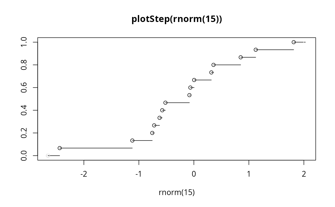
##-- Draw an Empirical CDF  (and see the default title ..)
plotStep(rnorm(15))


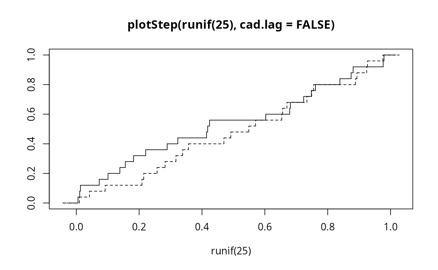
plotStep(runif(25), cad.lag=FALSE)
plotStep(runif(25), cad.lag=FALSE, add=TRUE, lty = 2)


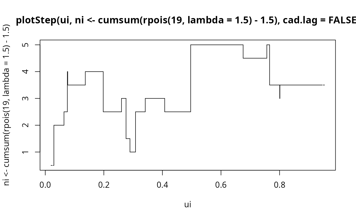
ui <- sort(runif(20))
plotStep(ui, ni <- cumsum(rpois(19, lambda=1.5) - 1.5), cad.lag = FALSE)

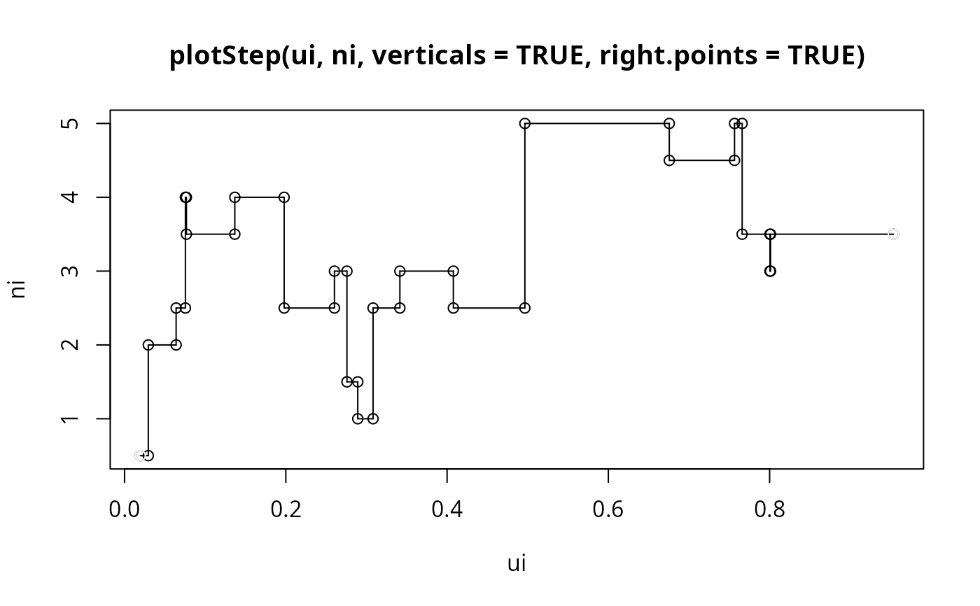
plotStep(ui, ni, verticals = TRUE, right.points = TRUE)


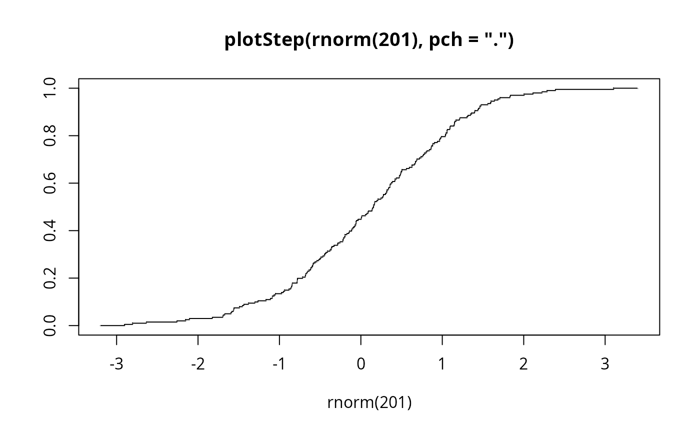
plotStep(rnorm(201), pch = '.') #- smaller points