Enhance Formula by Wrapping each Term, e.g., by "s(.)"

The main motivation for this function has been the easy construction of a “full GAM formula” from something as simple as Y ~ ..
The potential use is slightly more general.

Usage

wrapFormula(f, data, wrapString = "s(*)")

Arguments

f

the initial formula; typically something like Y ~ ..

data

data.frame to which the formula applies; see, formula or also gam or lm.

wrapString

character string, containing "*", specifying the wrapping expression to use.

Value

a formula very similar to f; just replacing each additive term by its wrapped version.

Note

There are limits for this to work correctly; notably the right hand side of the formula f should not be nested or otherwise complicated, rather typically just . as in the examples.

Author

Martin Maechler, May 2007.

See also

formula; gam from package mgcv (or also from package gam).

Examples

myF <- wrapFormula(Fertility ~ . , data = swiss)
myF # Fertility ~ s(Agriculture) + s(....) + ...
#> Fertility ~ s(Agriculture) + s(Examination) + s(Education) + 
#>     s(Catholic) + s(Infant.Mortality)
#> <environment: 0x5ec1bc013270>

if(require("mgcv")) {
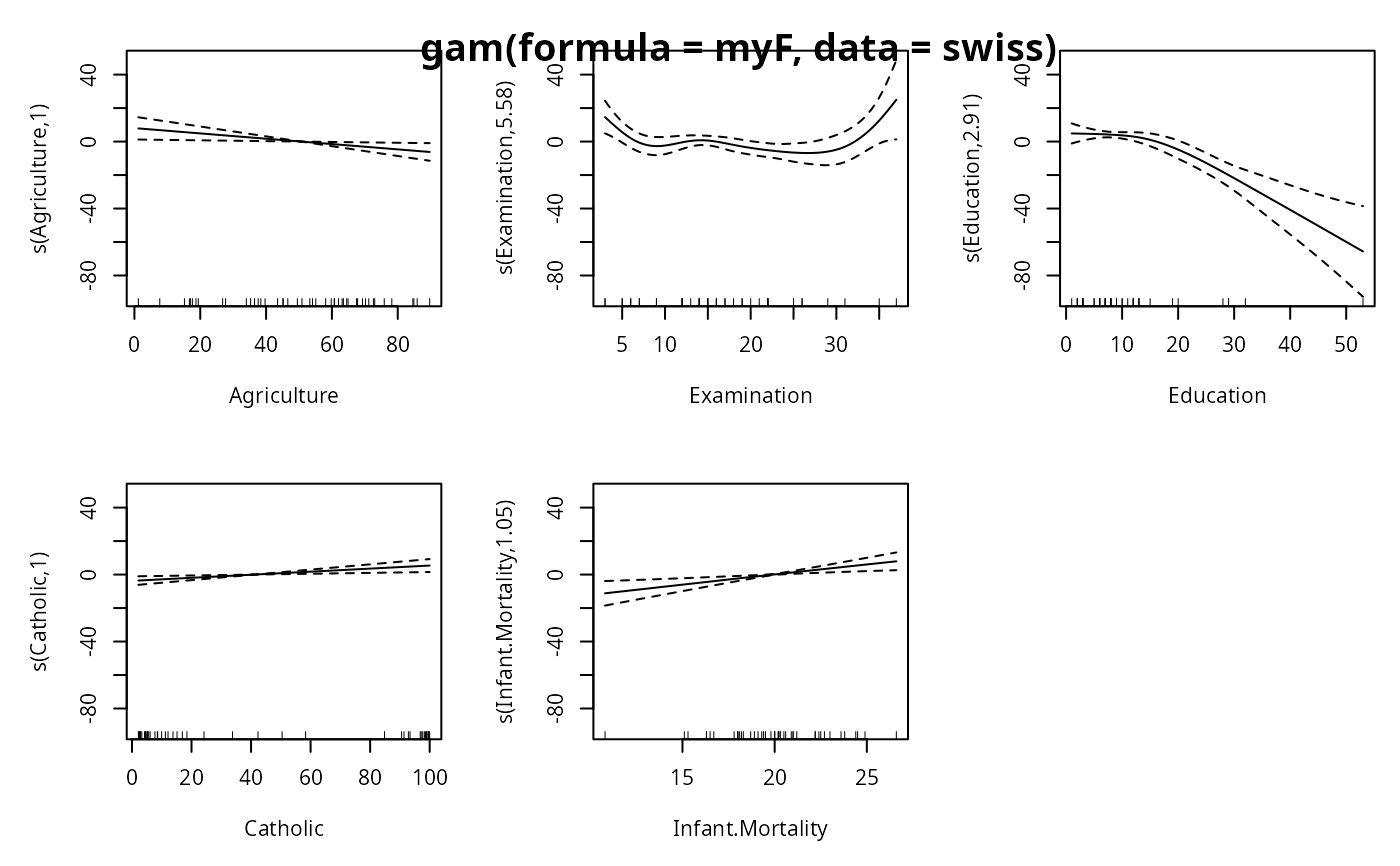
   m1 <- gam(myF, data = swiss)
   print( summary(m1) )
   plot(m1, pages = 1) ; title(format(m1$call), line= 2.5)
}
#> Loading required package: mgcv
#> Loading required package: nlme
#> This is mgcv 1.9-3. For overview type 'help("mgcv-package")'.
#> 
#> Family: gaussian 
#> Link function: identity 
#> 
#> Formula:
#> Fertility ~ s(Agriculture) + s(Examination) + s(Education) + 
#>     s(Catholic) + s(Infant.Mortality)
#> 
#> Parametric coefficients:
#>             Estimate Std. Error t value Pr(>|t|)    
#> (Intercept)   70.143      0.852    82.4   <2e-16 ***
#> ---
#> Signif. codes:  0 ‘***’ 0.001 ‘**’ 0.01 ‘*’ 0.05 ‘.’ 0.1 ‘ ’ 1
#> 
#> Approximate significance of smooth terms:
#>                      edf Ref.df     F p-value    
#> s(Agriculture)      1.00   1.00  5.59  0.0240 *  
#> s(Examination)      5.58   6.57  3.24  0.0111 *  
#> s(Education)        2.91   3.52 12.20 9.9e-06 ***
#> s(Catholic)         1.00   1.00  7.78  0.0086 ** 
#> s(Infant.Mortality) 1.05   1.10  9.14  0.0045 ** 
#> ---
#> Signif. codes:  0 ‘***’ 0.001 ‘**’ 0.01 ‘*’ 0.05 ‘.’ 0.1 ‘ ’ 1
#> 
#> R-sq.(adj) =  0.782   Deviance explained = 83.6%
#> GCV = 46.505  Scale est. = 34.09     n = 47


## other wrappers:
wrapFormula(Fertility ~ . , data = swiss, wrap = "lo(*)")
#> Fertility ~ lo(Agriculture) + lo(Examination) + lo(Education) + 
#>     lo(Catholic) + lo(Infant.Mortality)
#> <environment: 0x5ec1bc013270>
wrapFormula(Fertility ~ . , data = swiss, wrap = "poly(*, 4)")
#> Fertility ~ poly(Agriculture, 4) + poly(Examination, 4) + poly(Education, 
#>     4) + poly(Catholic, 4) + poly(Infant.Mortality, 4)
#> <environment: 0x5ec1bc013270>