Tabulate biomarker effects on survival by subgroup
Source:R/survival_biomarkers_subgroups.R
survival_biomarkers_subgroups.Rd![[Stable]](figures/lifecycle-stable.svg)
The tabulate_survival_biomarkers() function creates a layout element to tabulate the estimated effects of multiple
continuous biomarker variables on survival across subgroups, returning statistics including median survival time and
hazard ratio for each population subgroup. The table is created from df, a list of data frames returned by
extract_survival_biomarkers(), with the statistics to include specified via the vars parameter.
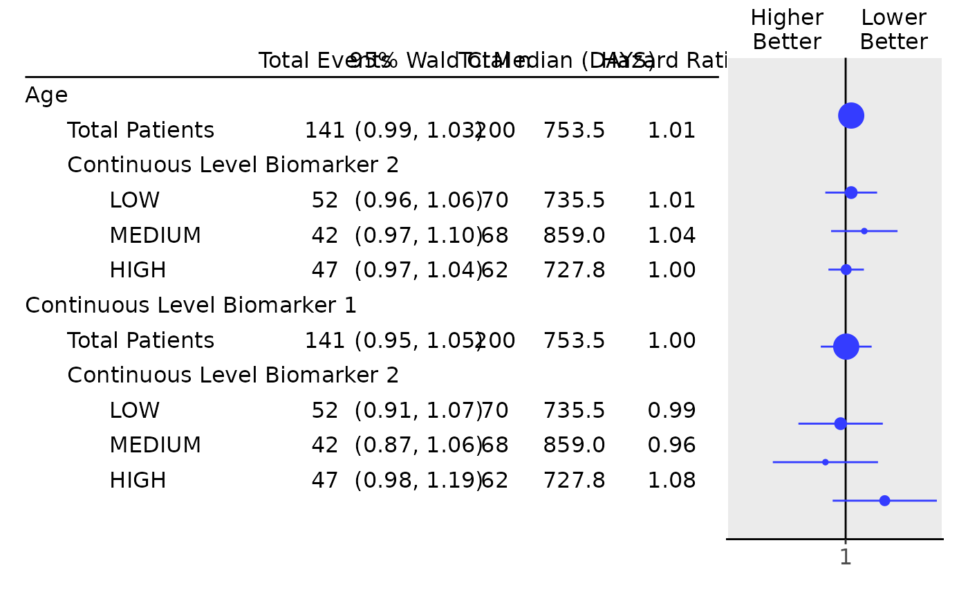
A forest plot can be created from the resulting table using the g_forest() function.
tabulate_survival_biomarkers(
  df,
  vars = c("n_tot", "n_tot_events", "median", "hr", "ci", "pval"),
  groups_lists = list(),
  control = control_coxreg(),
  label_all = lifecycle::deprecated(),
  time_unit = NULL,
  na_str = default_na_str(),
  .indent_mods = 0L
)
Arguments
- df
(
data.frame)
containing all analysis variables, as returned byextract_survival_biomarkers().- vars
(
character)
the names of statistics to be reported among:n_tot_events: Total number of events per group.n_tot: Total number of observations per group.median: Median survival time.hr: Hazard ratio.ci: Confidence interval of hazard ratio.pval: p-value of the effect. Note, one of the statisticsn_totandn_tot_events, as well as bothhrandciare required.
- groups_lists
(named
listoflist)
optionally contains for eachsubgroupsvariable a list, which specifies the new group levels via the names and the levels that belong to it in the character vectors that are elements of the list.- control
(
list)
a list of parameters as returned by the helper functioncontrol_coxreg().- label_all
![[Deprecated]](figures/lifecycle-deprecated.svg)
please assign thelabel_allparameter within theextract_survival_biomarkers()function when creatingdf.- time_unit
(
string)
label with unit of median survival time. DefaultNULLskips displaying unit.- na_str
(
string)
string used to replace allNAor empty values in the output.- .indent_mods
(named
integer)
indent modifiers for the labels. Defaults to 0, which corresponds to the unmodified default behavior. Can be negative.
Value
An rtables table summarizing biomarker effects on survival by subgroup.
Details
These functions create a layout starting from a data frame which contains the required statistics. The tables are then typically used as input for forest plots.
Functions
tabulate_survival_biomarkers(): Table-creating function which creates a table summarizing biomarker effects on survival by subgroup.
Note
In contrast to tabulate_survival_subgroups() this tabulation function does
not start from an input layout lyt. This is because internally the table is
created by combining multiple subtables.
See also
h_tab_surv_one_biomarker() which is used internally, extract_survival_biomarkers().
Examples
library(dplyr)

adtte <- tern_ex_adtte

# Save variable labels before data processing steps.
adtte_labels <- formatters::var_labels(adtte)

adtte_f <- adtte %>%
  filter(PARAMCD == "OS") %>%
  mutate(
    AVALU = as.character(AVALU),
    is_event = CNSR == 0
  )
labels <- c("AVALU" = adtte_labels[["AVALU"]], "is_event" = "Event Flag")
formatters::var_labels(adtte_f)[names(labels)] <- labels

# Typical analysis of two continuous biomarkers `BMRKR1` and `AGE`,
# in multiple regression models containing one covariate `RACE`,
# as well as one stratification variable `STRATA1`. The subgroups
# are defined by the levels of `BMRKR2`.

df <- extract_survival_biomarkers(
  variables = list(
    tte = "AVAL",
    is_event = "is_event",
    biomarkers = c("BMRKR1", "AGE"),
    strata = "STRATA1",
    covariates = "SEX",
    subgroups = "BMRKR2"
  ),
  label_all = "Total Patients",
  data = adtte_f
)
df
#>   biomarker              biomarker_label n_tot n_tot_events   median        hr
#> 1    BMRKR1 Continuous Level Biomarker 1   200          141 753.5176 1.0010939
#> 2       AGE                          Age   200          141 753.5176 1.0106406
#> 3    BMRKR1 Continuous Level Biomarker 1    70           52 735.4722 0.9905065
#> 4       AGE                          Age    70           52 735.4722 1.0106279
#> 5    BMRKR1 Continuous Level Biomarker 1    68           42 858.9952 0.9623210
#> 6       AGE                          Age    68           42 858.9952 1.0360765
#> 7    BMRKR1 Continuous Level Biomarker 1    62           47 727.8043 1.0770946
#> 8       AGE                          Age    62           47 727.8043 1.0009890
#>         lcl      ucl conf_level      pval     pval_label       subgroup    var
#> 1 0.9538978 1.050625       0.95 0.9646086 p-value (Wald) Total Patients    ALL
#> 2 0.9871004 1.034742       0.95 0.3787395 p-value (Wald) Total Patients    ALL
#> 3 0.9142220 1.073156       0.95 0.8155443 p-value (Wald)            LOW BMRKR2
#> 4 0.9621192 1.061582       0.95 0.6735773 p-value (Wald)            LOW BMRKR2
#> 5 0.8708694 1.063376       0.95 0.4509368 p-value (Wald)         MEDIUM BMRKR2
#> 6 0.9727439 1.103532       0.95 0.2707796 p-value (Wald)         MEDIUM BMRKR2
#> 7 0.9756250 1.189118       0.95 0.1412524 p-value (Wald)           HIGH BMRKR2
#> 8 0.9678535 1.035259       0.95 0.9541048 p-value (Wald)           HIGH BMRKR2
#>                      var_label row_type
#> 1               Total Patients  content
#> 2               Total Patients  content
#> 3 Continuous Level Biomarker 2 analysis
#> 4 Continuous Level Biomarker 2 analysis
#> 5 Continuous Level Biomarker 2 analysis
#> 6 Continuous Level Biomarker 2 analysis
#> 7 Continuous Level Biomarker 2 analysis
#> 8 Continuous Level Biomarker 2 analysis

# Here we group the levels of `BMRKR2` manually.
df_grouped <- extract_survival_biomarkers(
  variables = list(
    tte = "AVAL",
    is_event = "is_event",
    biomarkers = c("BMRKR1", "AGE"),
    strata = "STRATA1",
    covariates = "SEX",
    subgroups = "BMRKR2"
  ),
  data = adtte_f,
  groups_lists = list(
    BMRKR2 = list(
      "low" = "LOW",
      "low/medium" = c("LOW", "MEDIUM"),
      "low/medium/high" = c("LOW", "MEDIUM", "HIGH")
    )
  )
)
df_grouped
#>   biomarker              biomarker_label n_tot n_tot_events   median        hr
#> 1    BMRKR1 Continuous Level Biomarker 1   200          141 753.5176 1.0010939
#> 2       AGE                          Age   200          141 753.5176 1.0106406
#> 3    BMRKR1 Continuous Level Biomarker 1    70           52 735.4722 0.9905065
#> 4       AGE                          Age    70           52 735.4722 1.0106279
#> 5    BMRKR1 Continuous Level Biomarker 1   138           94 777.8929 0.9801709
#> 6       AGE                          Age   138           94 777.8929 1.0236283
#> 7    BMRKR1 Continuous Level Biomarker 1   200          141 753.5176 1.0010939
#> 8       AGE                          Age   200          141 753.5176 1.0106406
#>         lcl      ucl conf_level      pval     pval_label        subgroup    var
#> 1 0.9538978 1.050625       0.95 0.9646086 p-value (Wald)    All Patients    ALL
#> 2 0.9871004 1.034742       0.95 0.3787395 p-value (Wald)    All Patients    ALL
#> 3 0.9142220 1.073156       0.95 0.8155443 p-value (Wald)             low BMRKR2
#> 4 0.9621192 1.061582       0.95 0.6735773 p-value (Wald)             low BMRKR2
#> 5 0.9235465 1.040267       0.95 0.5094582 p-value (Wald)      low/medium BMRKR2
#> 6 0.9859367 1.062761       0.95 0.2224475 p-value (Wald)      low/medium BMRKR2
#> 7 0.9538978 1.050625       0.95 0.9646086 p-value (Wald) low/medium/high BMRKR2
#> 8 0.9871004 1.034742       0.95 0.3787395 p-value (Wald) low/medium/high BMRKR2
#>                      var_label row_type
#> 1                 All Patients  content
#> 2                 All Patients  content
#> 3 Continuous Level Biomarker 2 analysis
#> 4 Continuous Level Biomarker 2 analysis
#> 5 Continuous Level Biomarker 2 analysis
#> 6 Continuous Level Biomarker 2 analysis
#> 7 Continuous Level Biomarker 2 analysis
#> 8 Continuous Level Biomarker 2 analysis

## Table with default columns.
tabulate_survival_biomarkers(df)
#>                                  Total n   Total Events   Median   Hazard Ratio   95% Wald CI    p-value (Wald)
#> ———————————————————————————————————————————————————————————————————————————————————————————————————————————————
#> Age
#>   Total Patients                   200         141        753.5        1.01       (0.99, 1.03)       0.3787
#>   Continuous Level Biomarker 2
#>     LOW                            70           52        735.5        1.01       (0.96, 1.06)       0.6736
#>     MEDIUM                         68           42        859.0        1.04       (0.97, 1.10)       0.2708
#>     HIGH                           62           47        727.8        1.00       (0.97, 1.04)       0.9541
#> Continuous Level Biomarker 1
#>   Total Patients                   200         141        753.5        1.00       (0.95, 1.05)       0.9646
#>   Continuous Level Biomarker 2
#>     LOW                            70           52        735.5        0.99       (0.91, 1.07)       0.8155
#>     MEDIUM                         68           42        859.0        0.96       (0.87, 1.06)       0.4509
#>     HIGH                           62           47        727.8        1.08       (0.98, 1.19)       0.1413

## Table with a manually chosen set of columns: leave out "pval", reorder.
tab <- tabulate_survival_biomarkers(
  df = df,
  vars = c("n_tot_events", "ci", "n_tot", "median", "hr"),
  time_unit = as.character(adtte_f$AVALU[1])
)

## Finally produce the forest plot.
# \donttest{
g_forest(tab, xlim = c(0.8, 1.2))

# }
# }