Tabulate biomarker effects on binary response by subgroup

The tabulate_rsp_biomarkers() function creates a layout element to tabulate the estimated biomarker effects on a binary response endpoint across subgroups, returning statistics including response rate and odds ratio for each population subgroup. The table is created from df, a list of data frames returned by extract_rsp_biomarkers(), with the statistics to include specified via the vars parameter.

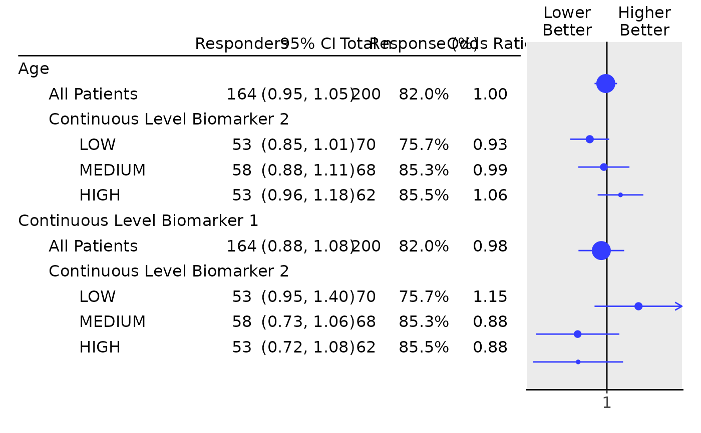
A forest plot can be created from the resulting table using the g_forest() function.

tabulate_rsp_biomarkers(
  df,
  vars = c("n_tot", "n_rsp", "prop", "or", "ci", "pval"),
  na_str = default_na_str(),
  ...,
  .stat_names = NULL,
  .formats = NULL,
  .labels = NULL,
  .indent_mods = NULL
)

Arguments

df

(data.frame)
containing all analysis variables, as returned by extract_rsp_biomarkers().

vars

(character)
the names of statistics to be reported among:

• n_tot: Total number of patients per group.

• n_rsp: Total number of responses per group.

• prop: Total response proportion per group.

• or: Odds ratio.

• ci: Confidence interval of odds ratio.

• pval: p-value of the effect. Note, the statistics n_tot, or and ci are required.

na_str

(string)
string used to replace all NA or empty values in the output.

...

additional arguments for the lower level functions.

.stat_names

(character)
names of the statistics that are passed directly to name single statistics (.stats). This option is visible when producing rtables::as_result_df() with make_ard = TRUE.

.formats

(named character or list)
formats for the statistics. See Details in analyze_vars for more information on the "auto" setting.

.labels

(named character)
labels for the statistics (without indent).

.indent_mods

(named integer)
indent modifiers for the labels. Defaults to 0, which corresponds to the unmodified default behavior. Can be negative.

Value

An rtables table summarizing biomarker effects on binary response by subgroup.

Details

These functions create a layout starting from a data frame which contains the required statistics. The tables are then typically used as input for forest plots.

Note

In contrast to tabulate_rsp_subgroups() this tabulation function does not start from an input layout lyt. This is because internally the table is created by combining multiple subtables.

See also

extract_rsp_biomarkers()

Examples

library(dplyr)
library(forcats)

adrs <- tern_ex_adrs
adrs_labels <- formatters::var_labels(adrs)

adrs_f <- adrs %>%
  filter(PARAMCD == "BESRSPI") %>%
  mutate(rsp = AVALC == "CR")
formatters::var_labels(adrs_f) <- c(adrs_labels, "Response")

df <- extract_rsp_biomarkers(
  variables = list(
    rsp = "rsp",
    biomarkers = c("BMRKR1", "AGE"),
    covariates = "SEX",
    subgroups = "BMRKR2"
  ),
  data = adrs_f
)

# \donttest{
## Table with default columns.
tabulate_rsp_biomarkers(df)
#>                                  Total n   Responders   Response (%)   Odds Ratio      95% CI      p-value (Wald)
#> —————————————————————————————————————————————————————————————————————————————————————————————————————————————————
#> Age                                                                                                              
#>   All Patients                     200        164          82.0%          1.00      (0.95, 1.05)       0.8530    
#>   Continuous Level Biomarker 2                                                                                   
#>     LOW                            70          53          75.7%          0.93      (0.85, 1.01)       0.0845    
#>     MEDIUM                         68          58          85.3%          0.99      (0.88, 1.11)       0.8190    
#>     HIGH                           62          53          85.5%          1.06      (0.96, 1.18)       0.2419    
#> Continuous Level Biomarker 1                                                                                     
#>   All Patients                     200        164          82.0%          0.98      (0.88, 1.08)       0.6353    
#>   Continuous Level Biomarker 2                                                                                   
#>     LOW                            70          53          75.7%          1.15      (0.95, 1.40)       0.1584    
#>     MEDIUM                         68          58          85.3%          0.88      (0.73, 1.06)       0.1700    
#>     HIGH                           62          53          85.5%          0.88      (0.72, 1.08)       0.2104    

## Table with a manually chosen set of columns: leave out "pval", reorder.
tab <- tabulate_rsp_biomarkers(
  df = df,
  vars = c("n_rsp", "ci", "n_tot", "prop", "or")
)

## Finally produce the forest plot.
g_forest(tab, xlim = c(0.7, 1.4))

# }