Truncated Multivariate Student t Density

This function provides the joint density function for the truncated multivariate Student t distribution with mean vector equal to mean, covariance matrix sigma, degrees of freedom parameter df and lower and upper truncation points lower and upper.

dtmvt(x, mean = rep(0, nrow(sigma)), sigma = diag(length(mean)), df = 1, 
lower = rep(-Inf, length = length(mean)), 
upper = rep(Inf, length = length(mean)), log = FALSE)

Arguments

x: Vector or matrix of quantiles. If x is a matrix, each row is taken to be a quantile.
mean: Mean vector, default is rep(0, nrow(sigma)).
sigma: Covariance matrix, default is diag(length(mean)).
df: degrees of freedom parameter
lower: Vector of lower truncation points, default is rep(-Inf, length = length(mean)).
upper: Vector of upper truncation points, default is rep( Inf, length = length(mean)).
log: Logical; if TRUE, densities d are given as log(d).

Details

The Truncated Multivariate Student t Distribution is a conditional Multivariate Student t distribution subject to (linear) constraints $a \le \bold{x} \le b$.

The density of the $p$-variate Multivariate Student t distribution with $\nu$ degrees of freedom is $$ f(\bold{x}) = \frac{\Gamma((\nu + p)/2)}{(\pi\nu)^{p/2} \Gamma(\nu/2) \|\Sigma\|^{1/2}} [ 1 + \frac{1}{\nu} (x - \mu)^T \Sigma^{-1} (x - \mu) ]^{- (\nu + p) / 2} $$ The density of the truncated distribution $f_{a,b}(x)$ with constraints $(a \le x \le b)$ is accordingly $$ f_{a,b}(x) = \frac{f(\bold{x})} {P(a \le x \le b)} $$

Value

a numeric vector with density values

References

Geweke, J. F. (1991) Efficient simulation from the multivariate normal and Student-t distributions subject to linear constraints and the evaluation of constraint probabilities. https://www.researchgate.net/publication/2335219_Efficient_Simulation_from_the_Multivariate_Normal_and_Student-t_Distributions_Subject_to_Linear_Constraints_and_the_Evaluation_of_Constraint_Probabilities

Samuel Kotz, Saralees Nadarajah (2004). Multivariate t Distributions and Their Applications. Cambridge University Press

Author

Stefan Wilhelm wilhelm@financial.com

Examples

# Example

x1 <- seq(-2, 3, by=0.1)
x2 <- seq(-2, 3, by=0.1)

mean <- c(0,0)
sigma <- matrix(c(1, -0.5, -0.5, 1), 2, 2)
lower <- c(-1,-1)


density <- function(x)
{
  z=dtmvt(x, mean=mean, sigma=sigma, lower=lower)
  z
}

fgrid <- function(x, y, f)
{
  z <- matrix(nrow=length(x), ncol=length(y))
  for(m in 1:length(x)){
    for(n in 1:length(y)){
      z[m,n] <- f(c(x[m], y[n]))
    }
  }
  z
}

# compute multivariate-t density d for grid
d <- fgrid(x1, x2, function(x) dtmvt(x, mean=mean, sigma=sigma, lower=lower))

# compute multivariate normal density d for grid
d2 <- fgrid(x1, x2, function(x) dtmvnorm(x, mean=mean, sigma=sigma, lower=lower))

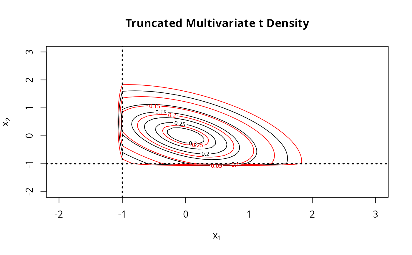
# plot density as contourplot
contour(x1, x2, d, nlevels=5, main="Truncated Multivariate t Density", 
    xlab=expression(x[1]), ylab=expression(x[2]))

contour(x1, x2, d2, nlevels=5, add=TRUE, col="red")
abline(v=-1, lty=3, lwd=2)
abline(h=-1, lty=3, lwd=2)