Fit ARMA Models to Time Series
arma.RdFit an ARMA model to a univariate time series by conditional least
squares. For exact maximum likelihood estimation see
arima0.
arma(x, order = c(1, 1), lag = NULL, coef = NULL,
     include.intercept = TRUE, series = NULL, qr.tol = 1e-07, ...)
Arguments
- x
a numeric vector or time series.
- order
a two dimensional integer vector giving the orders of the model to fit.
order[1]corresponds to the AR part andorder[2]to the MA part.- lag
a list with components
arandma. Each component is an integer vector, specifying the AR and MA lags that are included in the model. If both,orderandlag, are given, only the specification fromlagis used.- coef
If given this numeric vector is used as the initial estimate of the ARMA coefficients. The preliminary estimator suggested in Hannan and Rissanen (1982) is used for the default initialization.
- include.intercept
Should the model contain an intercept?
- series
name for the series. Defaults to
deparse(substitute(x)).- qr.tol
the
tolargument forqrwhen computing the asymptotic standard errors ofcoef.- ...
additional arguments for
optimwhen fitting the model.
Details
The following parametrization is used for the ARMA(p,q) model:
$$y[t] = a[0] + a[1]y[t-1] + \dots + a[p]y[t-p] + b[1]e[t-1] + \dots + b[q]e[t-q] + e[t],$$
where \(a[0]\) is set to zero if no intercept is included. By using
the argument lag, it is possible to fit a parsimonious submodel
by setting arbitrary \(a[i]\) and \(b[i]\) to zero.
arma uses optim to minimize the conditional
sum-of-squared errors. The gradient is computed, if it is needed, by
a finite-difference approximation. Default initialization is done by
fitting a pure high-order AR model (see ar.ols).
The estimated residuals are then used for computing a least squares
estimator of the full ARMA model. See Hannan and Rissanen (1982) for
details.
Value
A list of class "arma" with the following elements:
- lag
the lag specification of the fitted model.
- coef
estimated ARMA coefficients for the fitted model.
- css
the conditional sum-of-squared errors.
- n.used
the number of observations of
x.- residuals
the series of residuals.
- fitted.values
the fitted series.
- series
the name of the series
x.- frequency
the frequency of the series
x.- call
the call of the
armafunction.- vcov
estimate of the asymptotic-theory covariance matrix for the coefficient estimates.
- convergence
The
convergenceinteger code fromoptim.- include.intercept
Does the model contain an intercept?
References
E. J. Hannan and J. Rissanen (1982): Recursive Estimation of Mixed Autoregressive-Moving Average Order. Biometrika 69, 81–94.
See also
summary.arma for summarizing ARMA model fits;
arma-methods for further methods;
arima0, ar.
Examples
data(tcm)
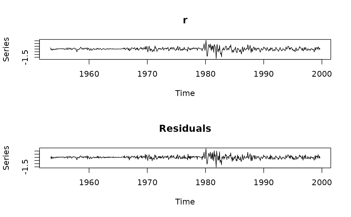
r <- diff(tcm10y)
summary(r.arma <- arma(r, order = c(1, 0)))
#>
#> Call:
#> arma(x = r, order = c(1, 0))
#>
#> Model:
#> ARMA(1,0)
#>
#> Residuals:
#> Min 1Q Median 3Q Max
#> -1.707400 -0.116059 0.006282 0.128118 1.471796
#>
#> Coefficient(s):
#> Estimate Std. Error t value Pr(>|t|)
#> ar1 0.328972 0.039991 8.226 2.22e-16 ***
#> intercept 0.003325 0.011430 0.291 0.771
#> ---
#> Signif. codes: 0 ‘***’ 0.001 ‘**’ 0.01 ‘*’ 0.05 ‘.’ 0.1 ‘ ’ 1
#>
#> Fit:
#> sigma^2 estimated as 0.07287, Conditional Sum-of-Squares = 40.44, AIC = 125.89
#>
summary(r.arma <- arma(r, order = c(2, 0)))
#>
#> Call:
#> arma(x = r, order = c(2, 0))
#>
#> Model:
#> ARMA(2,0)
#>
#> Residuals:
#> Min 1Q Median 3Q Max
#> -1.603801 -0.117037 0.002274 0.129126 1.376261
#>
#> Coefficient(s):
#> Estimate Std. Error t value Pr(>|t|)
#> ar1 0.40790 0.04114 9.915 < 2e-16 ***
#> ar2 -0.23962 0.04113 -5.826 5.67e-09 ***
#> intercept 0.00420 0.01111 0.378 0.705
#> ---
#> Signif. codes: 0 ‘***’ 0.001 ‘**’ 0.01 ‘*’ 0.05 ‘.’ 0.1 ‘ ’ 1
#>
#> Fit:
#> sigma^2 estimated as 0.06881, Conditional Sum-of-Squares = 38.12, AIC = 95.94
#>
summary(r.arma <- arma(r, order = c(0, 1)))
#>
#> Call:
#> arma(x = r, order = c(0, 1))
#>
#> Model:
#> ARMA(0,1)
#>
#> Residuals:
#> Min 1Q Median 3Q Max
#> -1.590634 -0.118433 -0.000165 0.129751 1.339717
#>
#> Coefficient(s):
#> Estimate Std. Error t value Pr(>|t|)
#> ma1 0.506871 0.042113 12.036 <2e-16 ***
#> intercept 0.005287 0.016632 0.318 0.751
#> ---
#> Signif. codes: 0 ‘***’ 0.001 ‘**’ 0.01 ‘*’ 0.05 ‘.’ 0.1 ‘ ’ 1
#>
#> Fit:
#> sigma^2 estimated as 0.06811, Conditional Sum-of-Squares = 37.8, AIC = 88.21
#>
summary(r.arma <- arma(r, order = c(0, 2)))
#>
#> Call:
#> arma(x = r, order = c(0, 2))
#>
#> Model:
#> ARMA(0,2)
#>
#> Residuals:
#> Min 1Q Median 3Q Max
#> -1.5497077 -0.1224297 0.0009082 0.1343164 1.3639450
#>
#> Coefficient(s):
#> Estimate Std. Error t value Pr(>|t|)
#> ma1 0.449184 0.042387 10.597 <2e-16 ***
#> ma2 -0.117937 0.042662 -2.764 0.0057 **
#> intercept 0.004701 0.014613 0.322 0.7477
#> ---
#> Signif. codes: 0 ‘***’ 0.001 ‘**’ 0.01 ‘*’ 0.05 ‘.’ 0.1 ‘ ’ 1
#>
#> Fit:
#> sigma^2 estimated as 0.0673, Conditional Sum-of-Squares = 37.28, AIC = 83.58
#>
summary(r.arma <- arma(r, order = c(1, 1)))
#>
#> Call:
#> arma(x = r, order = c(1, 1))
#>
#> Model:
#> ARMA(1,1)
#>
#> Residuals:
#> Min 1Q Median 3Q Max
#> -1.5529214 -0.1189386 0.0001515 0.1337559 1.3663775
#>
#> Coefficient(s):
#> Estimate Std. Error t value Pr(>|t|)
#> ar1 -0.202320 0.074961 -2.699 0.00695 **
#> ma1 0.658111 0.056927 11.561 < 2e-16 ***
#> intercept 0.006799 0.018195 0.374 0.70866
#> ---
#> Signif. codes: 0 ‘***’ 0.001 ‘**’ 0.01 ‘*’ 0.05 ‘.’ 0.1 ‘ ’ 1
#>
#> Fit:
#> sigma^2 estimated as 0.06731, Conditional Sum-of-Squares = 37.35, AIC = 83.62
#>
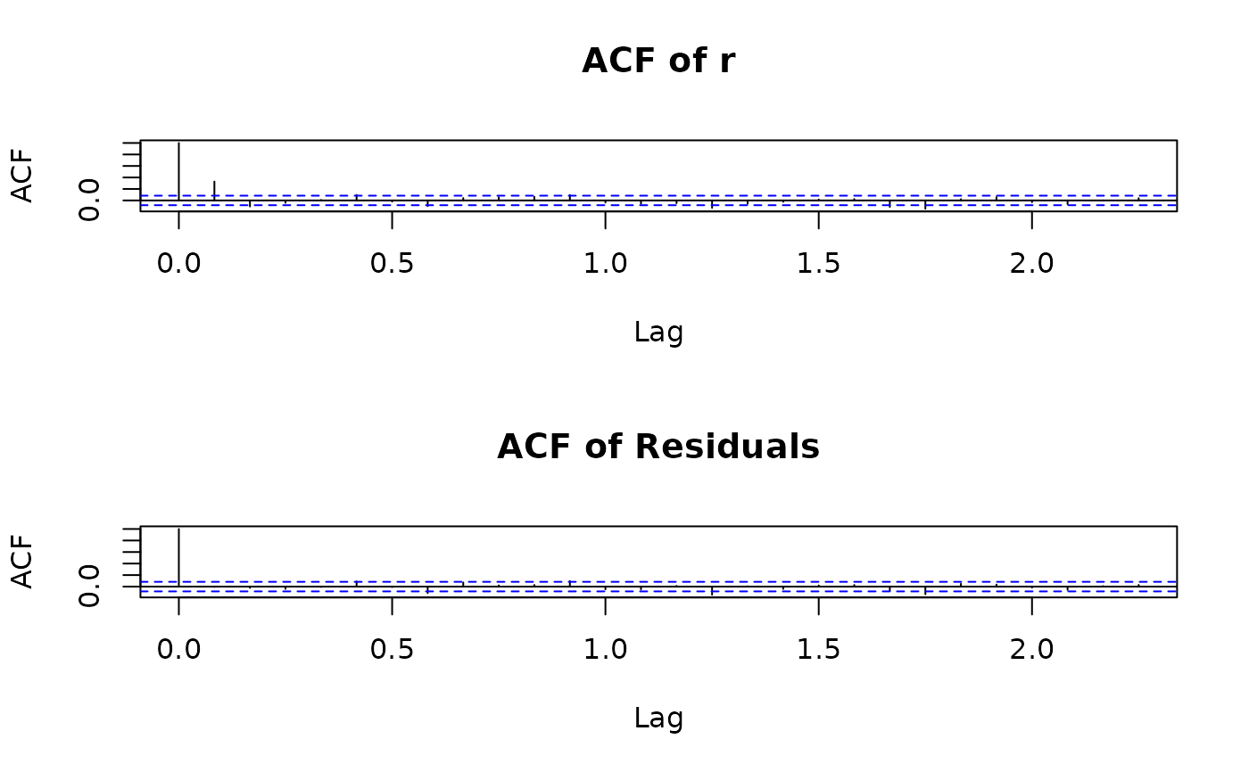
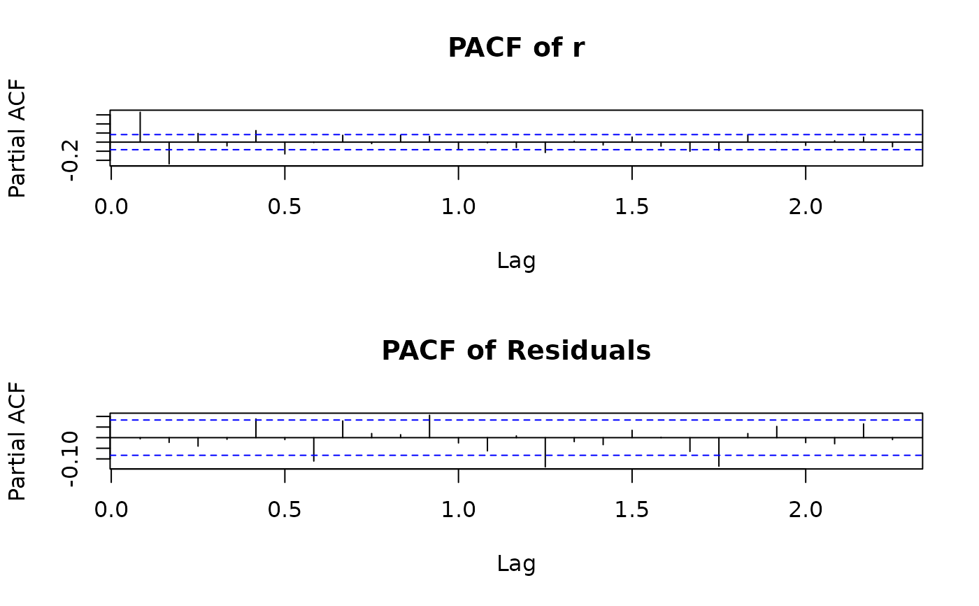
plot(r.arma)
 data(nino)
s <- nino3.4
summary(s.arma <- arma(s, order=c(20,0)))
#> Warning: Hessian negative-semidefinite
#> Warning: NaNs produced
#> Warning: NaNs produced
#>
#> Call:
#> arma(x = s, order = c(20, 0))
#>
#> Model:
#> ARMA(20,0)
#>
#> Residuals:
#> Min 1Q Median 3Q Max
#> -1.378647 -0.223040 0.007358 0.215996 1.103511
#>
#> Coefficient(s):
#> Estimate Std. Error t value Pr(>|t|)
#> ar1 1.10163 0.76719 1.436 0.151
#> ar2 -0.05461 0.78209 -0.070 0.944
#> ar3 -0.17718 0.32569 -0.544 0.586
#> ar4 0.07072 NaN NaN NaN
#> ar5 -0.05292 NaN NaN NaN
#> ar6 0.06743 0.26705 0.253 0.801
#> ar7 -0.17060 0.38307 -0.445 0.656
#> ar8 -0.03509 0.59151 -0.059 0.953
#> ar9 0.03326 NaN NaN NaN
#> ar10 0.14149 0.49846 0.284 0.777
#> ar11 0.01597 NaN NaN NaN
#> ar12 0.16400 NaN NaN NaN
#> ar13 -0.22467 0.03743 -6.003 1.94e-09 ***
#> ar14 -0.01355 0.03359 -0.404 0.687
#> ar15 -0.04530 0.04226 -1.072 0.284
#> ar16 -0.18815 NaN NaN NaN
#> ar17 0.20923 NaN NaN NaN
#> ar18 0.07387 NaN NaN NaN
#> ar19 -0.13363 NaN NaN NaN
#> ar20 0.05234 0.01311 3.992 6.54e-05 ***
#> intercept 4.46824 0.73499 6.079 1.21e-09 ***
#> ---
#> Signif. codes: 0 ‘***’ 0.001 ‘**’ 0.01 ‘*’ 0.05 ‘.’ 0.1 ‘ ’ 1
#>
#> Fit:
#> sigma^2 estimated as 0.1079, Conditional Sum-of-Squares = 62.24, AIC = 407.41
#>
summary(s.arma
<- arma(s, lag=list(ar=c(1,3,7,10,12,13,16,17,19),ma=NULL)))
#> Warning: order is ignored
#> Warning: Hessian negative-semidefinite
#> Warning: NaNs produced
#> Warning: NaNs produced
#>
#> Call:
#> arma(x = s, lag = list(ar = c(1, 3, 7, 10, 12, 13, 16, 17, 19), ma = NULL))
#>
#> Model:
#> ARMA(19,0)
#>
#> Residuals:
#> Min 1Q Median 3Q Max
#> -1.360875 -0.230887 0.005043 0.226822 1.090989
#>
#> Coefficient(s):
#> Estimate Std. Error t value Pr(>|t|)
#> ar1 1.07772 NaN NaN NaN
#> ar3 -0.16942 NaN NaN NaN
#> ar7 -0.13913 NaN NaN NaN
#> ar10 0.16459 0.93090 0.177 0.860
#> ar12 0.20472 0.03502 5.846 5.04e-09 ***
#> ar13 -0.29976 NaN NaN NaN
#> ar16 -0.21637 0.04645 -4.659 3.18e-06 ***
#> ar17 0.25139 0.35034 0.718 0.473
#> ar19 -0.04510 NaN NaN NaN
#> intercept 4.61896 NaN NaN NaN
#> ---
#> Signif. codes: 0 ‘***’ 0.001 ‘**’ 0.01 ‘*’ 0.05 ‘.’ 0.1 ‘ ’ 1
#>
#> Fit:
#> sigma^2 estimated as 0.1094, Conditional Sum-of-Squares = 63.24, AIC = 393.87
#>
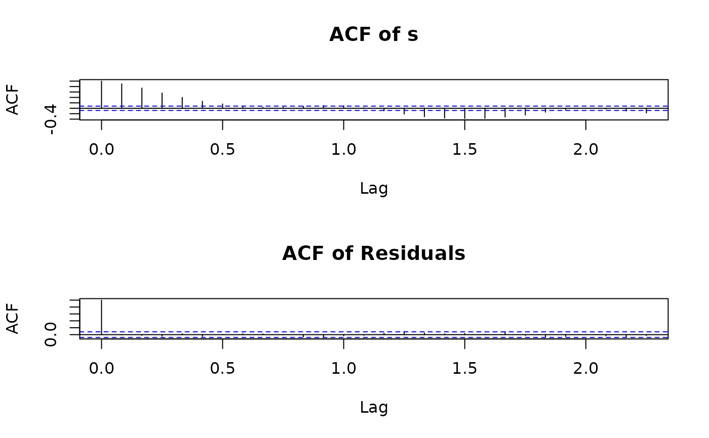
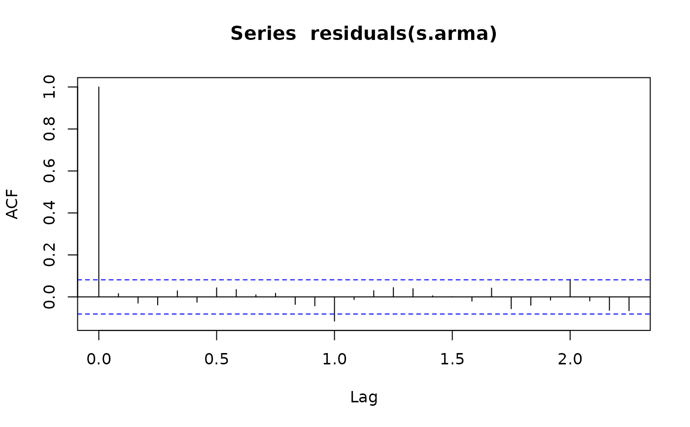
acf(residuals(s.arma), na.action=na.remove)
data(nino)
s <- nino3.4
summary(s.arma <- arma(s, order=c(20,0)))
#> Warning: Hessian negative-semidefinite
#> Warning: NaNs produced
#> Warning: NaNs produced
#>
#> Call:
#> arma(x = s, order = c(20, 0))
#>
#> Model:
#> ARMA(20,0)
#>
#> Residuals:
#> Min 1Q Median 3Q Max
#> -1.378647 -0.223040 0.007358 0.215996 1.103511
#>
#> Coefficient(s):
#> Estimate Std. Error t value Pr(>|t|)
#> ar1 1.10163 0.76719 1.436 0.151
#> ar2 -0.05461 0.78209 -0.070 0.944
#> ar3 -0.17718 0.32569 -0.544 0.586
#> ar4 0.07072 NaN NaN NaN
#> ar5 -0.05292 NaN NaN NaN
#> ar6 0.06743 0.26705 0.253 0.801
#> ar7 -0.17060 0.38307 -0.445 0.656
#> ar8 -0.03509 0.59151 -0.059 0.953
#> ar9 0.03326 NaN NaN NaN
#> ar10 0.14149 0.49846 0.284 0.777
#> ar11 0.01597 NaN NaN NaN
#> ar12 0.16400 NaN NaN NaN
#> ar13 -0.22467 0.03743 -6.003 1.94e-09 ***
#> ar14 -0.01355 0.03359 -0.404 0.687
#> ar15 -0.04530 0.04226 -1.072 0.284
#> ar16 -0.18815 NaN NaN NaN
#> ar17 0.20923 NaN NaN NaN
#> ar18 0.07387 NaN NaN NaN
#> ar19 -0.13363 NaN NaN NaN
#> ar20 0.05234 0.01311 3.992 6.54e-05 ***
#> intercept 4.46824 0.73499 6.079 1.21e-09 ***
#> ---
#> Signif. codes: 0 ‘***’ 0.001 ‘**’ 0.01 ‘*’ 0.05 ‘.’ 0.1 ‘ ’ 1
#>
#> Fit:
#> sigma^2 estimated as 0.1079, Conditional Sum-of-Squares = 62.24, AIC = 407.41
#>
summary(s.arma
<- arma(s, lag=list(ar=c(1,3,7,10,12,13,16,17,19),ma=NULL)))
#> Warning: order is ignored
#> Warning: Hessian negative-semidefinite
#> Warning: NaNs produced
#> Warning: NaNs produced
#>
#> Call:
#> arma(x = s, lag = list(ar = c(1, 3, 7, 10, 12, 13, 16, 17, 19), ma = NULL))
#>
#> Model:
#> ARMA(19,0)
#>
#> Residuals:
#> Min 1Q Median 3Q Max
#> -1.360875 -0.230887 0.005043 0.226822 1.090989
#>
#> Coefficient(s):
#> Estimate Std. Error t value Pr(>|t|)
#> ar1 1.07772 NaN NaN NaN
#> ar3 -0.16942 NaN NaN NaN
#> ar7 -0.13913 NaN NaN NaN
#> ar10 0.16459 0.93090 0.177 0.860
#> ar12 0.20472 0.03502 5.846 5.04e-09 ***
#> ar13 -0.29976 NaN NaN NaN
#> ar16 -0.21637 0.04645 -4.659 3.18e-06 ***
#> ar17 0.25139 0.35034 0.718 0.473
#> ar19 -0.04510 NaN NaN NaN
#> intercept 4.61896 NaN NaN NaN
#> ---
#> Signif. codes: 0 ‘***’ 0.001 ‘**’ 0.01 ‘*’ 0.05 ‘.’ 0.1 ‘ ’ 1
#>
#> Fit:
#> sigma^2 estimated as 0.1094, Conditional Sum-of-Squares = 63.24, AIC = 393.87
#>
acf(residuals(s.arma), na.action=na.remove)
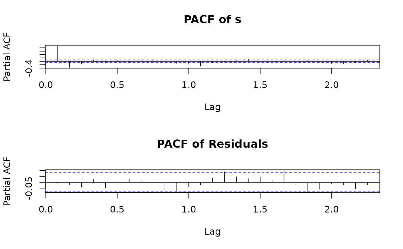
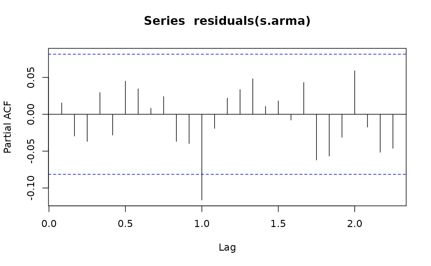
 pacf(residuals(s.arma), na.action=na.remove)
 summary(s.arma
<- arma(s, lag=list(ar=c(1,3,7,10,12,13,16,17,19),ma=12)))
#> Warning: order is ignored
#> Warning: Hessian negative-semidefinite
#> Warning: NaNs produced
#> Warning: NaNs produced
#>
#> Call:
#> arma(x = s, lag = list(ar = c(1, 3, 7, 10, 12, 13, 16, 17, 19), ma = 12))
#>
#> Model:
#> ARMA(19,12)
#>
#> Residuals:
#> Min 1Q Median 3Q Max
#> -1.339941 -0.209727 0.001678 0.224448 1.065923
#>
#> Coefficient(s):
#> Estimate Std. Error t value Pr(>|t|)
#> ar1 1.0664384 0.3819735 2.792 0.00524 **
#> ar3 -0.1539386 0.9061264 -0.170 0.86510
#> ar7 -0.1219358 0.2101116 -0.580 0.56169
#> ar10 0.1268904 0.3365205 0.377 0.70612
#> ar12 0.4622781 NaN NaN NaN
#> ar13 -0.5361871 0.0124042 -43.226 < 2e-16 ***
#> ar16 -0.1819534 NaN NaN NaN
#> ar17 0.2485878 0.0074805 33.231 < 2e-16 ***
#> ar19 -0.0446280 0.0005893 -75.725 < 2e-16 ***
#> ma12 -0.3637566 NaN NaN NaN
#> intercept 3.6229256 0.3555290 10.190 < 2e-16 ***
#> ---
#> Signif. codes: 0 ‘***’ 0.001 ‘**’ 0.01 ‘*’ 0.05 ‘.’ 0.1 ‘ ’ 1
#>
#> Fit:
#> sigma^2 estimated as 0.103, Conditional Sum-of-Squares = 59.54, AIC = 359.84
#>
summary(s.arma
<- arma(s, lag=list(ar=c(1,3,7,10,12,13,16,17),ma=12)))
#> Warning: order is ignored
#> Warning: Hessian negative-semidefinite
#> Warning: NaNs produced
#> Warning: NaNs produced
#>
#> Call:
#> arma(x = s, lag = list(ar = c(1, 3, 7, 10, 12, 13, 16, 17), ma = 12))
#>
#> Model:
#> ARMA(17,12)
#>
#> Residuals:
#> Min 1Q Median 3Q Max
#> -1.27924 -0.19931 0.01423 0.22825 1.08027
#>
#> Coefficient(s):
#> Estimate Std. Error t value Pr(>|t|)
#> ar1 1.056795 0.052722 20.045 < 2e-16 ***
#> ar3 -0.107234 0.297456 -0.361 0.718471
#> ar7 -0.154822 NaN NaN NaN
#> ar10 0.144584 0.578532 0.250 0.802653
#> ar12 0.535436 1.188918 0.450 0.652454
#> ar13 -0.641332 NaN NaN NaN
#> ar16 -0.142785 0.040465 -3.529 0.000418 ***
#> ar17 0.197391 0.003327 59.325 < 2e-16 ***
#> ma12 -0.430086 0.112346 -3.828 0.000129 ***
#> intercept 3.015824 NaN NaN NaN
#> ---
#> Signif. codes: 0 ‘***’ 0.001 ‘**’ 0.01 ‘*’ 0.05 ‘.’ 0.1 ‘ ’ 1
#>
#> Fit:
#> sigma^2 estimated as 0.1023, Conditional Sum-of-Squares = 59.37, AIC = 353.98
#>
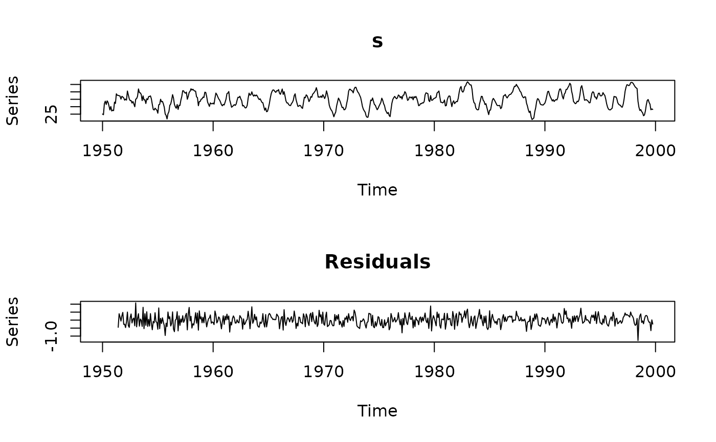
plot(s.arma)
summary(s.arma
<- arma(s, lag=list(ar=c(1,3,7,10,12,13,16,17,19),ma=12)))
#> Warning: order is ignored
#> Warning: Hessian negative-semidefinite
#> Warning: NaNs produced
#> Warning: NaNs produced
#>
#> Call:
#> arma(x = s, lag = list(ar = c(1, 3, 7, 10, 12, 13, 16, 17, 19), ma = 12))
#>
#> Model:
#> ARMA(19,12)
#>
#> Residuals:
#> Min 1Q Median 3Q Max
#> -1.339941 -0.209727 0.001678 0.224448 1.065923
#>
#> Coefficient(s):
#> Estimate Std. Error t value Pr(>|t|)
#> ar1 1.0664384 0.3819735 2.792 0.00524 **
#> ar3 -0.1539386 0.9061264 -0.170 0.86510
#> ar7 -0.1219358 0.2101116 -0.580 0.56169
#> ar10 0.1268904 0.3365205 0.377 0.70612
#> ar12 0.4622781 NaN NaN NaN
#> ar13 -0.5361871 0.0124042 -43.226 < 2e-16 ***
#> ar16 -0.1819534 NaN NaN NaN
#> ar17 0.2485878 0.0074805 33.231 < 2e-16 ***
#> ar19 -0.0446280 0.0005893 -75.725 < 2e-16 ***
#> ma12 -0.3637566 NaN NaN NaN
#> intercept 3.6229256 0.3555290 10.190 < 2e-16 ***
#> ---
#> Signif. codes: 0 ‘***’ 0.001 ‘**’ 0.01 ‘*’ 0.05 ‘.’ 0.1 ‘ ’ 1
#>
#> Fit:
#> sigma^2 estimated as 0.103, Conditional Sum-of-Squares = 59.54, AIC = 359.84
#>
summary(s.arma
<- arma(s, lag=list(ar=c(1,3,7,10,12,13,16,17),ma=12)))
#> Warning: order is ignored
#> Warning: Hessian negative-semidefinite
#> Warning: NaNs produced
#> Warning: NaNs produced
#>
#> Call:
#> arma(x = s, lag = list(ar = c(1, 3, 7, 10, 12, 13, 16, 17), ma = 12))
#>
#> Model:
#> ARMA(17,12)
#>
#> Residuals:
#> Min 1Q Median 3Q Max
#> -1.27924 -0.19931 0.01423 0.22825 1.08027
#>
#> Coefficient(s):
#> Estimate Std. Error t value Pr(>|t|)
#> ar1 1.056795 0.052722 20.045 < 2e-16 ***
#> ar3 -0.107234 0.297456 -0.361 0.718471
#> ar7 -0.154822 NaN NaN NaN
#> ar10 0.144584 0.578532 0.250 0.802653
#> ar12 0.535436 1.188918 0.450 0.652454
#> ar13 -0.641332 NaN NaN NaN
#> ar16 -0.142785 0.040465 -3.529 0.000418 ***
#> ar17 0.197391 0.003327 59.325 < 2e-16 ***
#> ma12 -0.430086 0.112346 -3.828 0.000129 ***
#> intercept 3.015824 NaN NaN NaN
#> ---
#> Signif. codes: 0 ‘***’ 0.001 ‘**’ 0.01 ‘*’ 0.05 ‘.’ 0.1 ‘ ’ 1
#>
#> Fit:
#> sigma^2 estimated as 0.1023, Conditional Sum-of-Squares = 59.37, AIC = 353.98
#>
plot(s.arma)