Principal Response Curves for Treatments with Repeated Observations

Principal Response Curves (PRC) are a special case of Redundancy Analysis (rda) for multivariate responses in repeated observation design. They were originally suggested for ecological communities. They should be easier to interpret than traditional constrained ordination. They can also be used to study how the effects of a factor A depend on the levels of a factor B, that is A + A:B, in a multivariate response experiment.

prc(response, treatment, time, ...)
# S3 method for class 'prc'
summary(object, axis = 1, scaling = "sites", const,
        digits = 4, correlation = FALSE, ...)
# S3 method for class 'prc'
plot(x, species = TRUE, select, scaling = "symmetric",
     axis = 1, correlation = FALSE, const, type = "l", xlab, ylab, ylim,
     lty = 1:5, col = 1:6, pch, legpos, cex = 0.8, ...)

Arguments

response

Multivariate response data. Typically these are community (species) data. If the data are counts, they probably should be log transformed prior to the analysis.

treatment

A factor for treatments.

time

An unordered factor defining the observations times in the repeated design.

object, x

An prc result object.

axis

Axis shown (only one axis can be selected).

scaling

Scaling of species scores, identical to the scaling in scores.rda.

The type of scores can also be specified as one of "none", "sites", "species", or "symmetric", which correspond to the values 0, 1, 2, and 3 respectively. Argument correlation can be used in combination with these character descriptions to get the corresponding negative value.

const

General scaling constant for species scores (see scores.rda for details). Lower values will reduce the range of species scores, but will not influence the regression coefficients.

digits

Number of significant digits displayed.

correlation

logical; if scaling is a character description of the scaling type, correlation can be used to select correlation-like scores for PCA. See argument scaling for details.

species

Display species scores.

select

Vector to select displayed species. This can be a vector of indices or a logical vector which is TRUE for the selected species

type

Type of plot: "l" for lines, "p" for points or "b" for both.

xlab, ylab

Text to replace default axis labels.

ylim

Limits for the vertical axis.

lty, col, pch

Line type, colour and plotting characters (defaults supplied).

legpos

The position of the legend. A guess is made if this is not supplied, and NA will suppress legend.

cex

Character expansion for symbols and species labels.

...

Other parameters passed to functions.

Details

PRC is a special case of rda with a single factor for treatment and a single factor for time points in repeated observations. In vegan, the corresponding rda model is defined as rda(response ~ treatment * time + Condition(time)). Since the time appears twice in the model formula, its main effects will be aliased, and only the main effect of treatment and interaction terms are available, and will be used in PRC. Instead of usual multivariate ordination diagrams, PRC uses canonical (regression) coefficients and species scores for a single axis. All that the current functions do is to provide a special summary and plot methods that display the rda results in the PRC fashion. The current version only works with default contrasts (contr.treatment) in which the coefficients are contrasts against the first level, and the levels must be arranged so that the first level is the control (or a baseline). If necessary, you must change the baseline level with function relevel.

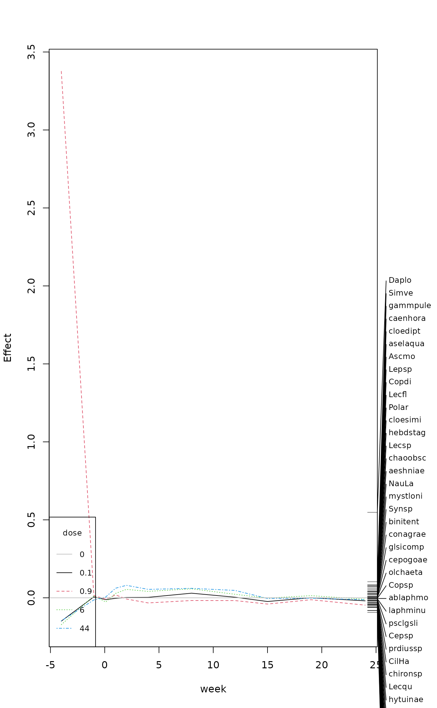
Function summary prints the species scores and the coefficients. Function plot plots coefficients against time using matplot, and has similar defaults. The graph (and PRC) is meaningful only if the first treatment level is the control, as the results are contrasts to the first level when unordered factors are used. The plot also displays species scores on the right vertical axis using function linestack. Typically the number of species is so high that not all can be displayed with the default settings, but users can reduce character size or padding (air) in linestack, or select only a subset of the species. A legend will be displayed unless suppressed with legpos = NA, and the functions tries to guess where to put the legend if legpos is not supplied.

Value

The function is a special case of rda and returns its result object (see cca.object). However, a special summary and plot methods display returns differently than in rda.

References

van den Brink, P.J. & ter Braak, C.J.F. (1999). Principal response curves: Analysis of time-dependent multivariate responses of biological community to stress. Environmental Toxicology and Chemistry, 18, 138–148.

Author

Jari Oksanen and Cajo ter Braak

Warning

The first level of treatment must be the control: use function relevel to guarantee the correct reference level. The current version will ignore user setting of contrasts and always use treatment contrasts (contr.treatment). The time must be an unordered factor.

Examples

## Chlorpyrifos experiment and experimental design: Pesticide
## treatment in ditches (replicated) and followed over from 4 weeks
## before to 24 weeks after exposure 
data(pyrifos)
week <- gl(11, 12, labels=c(-4, -1, 0.1, 1, 2, 4, 8, 12, 15, 19, 24))
dose <- factor(rep(c(0.1, 0, 0, 0.9, 0, 44, 6, 0.1, 44, 0.9, 0, 6), 11))
ditch <- gl(12, 1, length=132)

## IGNORE_RDIFF_BEGIN
## PRC
mod <- prc(pyrifos, dose, week)
mod            # RDA
#> 
#> Call: prc(response = pyrifos, treatment = dose, time = week)
#> 
#>                Inertia Proportion Rank
#> Total         288.9920     1.0000     
#> Conditional    63.3493     0.2192   10
#> Constrained    96.6837     0.3346   44
#> Unconstrained 128.9589     0.4462   77
#> 
#> Inertia is variance
#> 
#> Eigenvalues for constrained axes:
#>   RDA1   RDA2   RDA3   RDA4   RDA5   RDA6   RDA7   RDA8   RDA9  RDA10  RDA11 
#> 25.282  8.297  6.044  4.766  4.148  3.857  3.587  3.334  3.087  2.551  2.466 
#>  RDA12  RDA13  RDA14  RDA15  RDA16  RDA17  RDA18  RDA19  RDA20  RDA21  RDA22 
#>  2.209  2.129  1.941  1.799  1.622  1.579  1.440  1.398  1.284  1.211  1.133 
#>  RDA23  RDA24  RDA25  RDA26  RDA27  RDA28  RDA29  RDA30  RDA31  RDA32  RDA33 
#>  1.001  0.923  0.862  0.788  0.750  0.712  0.685  0.611  0.584  0.537  0.516 
#>  RDA34  RDA35  RDA36  RDA37  RDA38  RDA39  RDA40  RDA41  RDA42  RDA43  RDA44 
#>  0.442  0.417  0.404  0.368  0.340  0.339  0.306  0.279  0.271  0.205  0.179 
#> 
#> Eigenvalues for unconstrained axes:
#>    PC1    PC2    PC3    PC4    PC5    PC6    PC7    PC8 
#> 17.156  9.189  7.585  6.064  5.730  4.843  4.518  4.105 
#> (Showing 8 of 77 unconstrained eigenvalues)
#> 
summary(mod)   # PRC
#> 
#> Call:
#> prc(response = pyrifos, treatment = dose, time = week) 
#> Species scores:
#>      Simve      Daplo      Cerpu      Alogu      Aloco      Alore      Aloaf 
#>  0.1894282  1.0077690  9.9019576 -9.5106649  0.0050655 -0.0473220  0.1639303 
#>      Copsp      Ostsp      Slyla      Acrha      Aloex      Chysp      Alona 
#> -0.0061003 -0.0915237  0.1519611  0.0703536  0.0176863 -0.0062581 -0.0009135 
#>      Plead      Oxyte      Grate      Copdi      NauLa      CilHa      Strvi 
#>  0.0422777 -0.0123496 -0.0158249  0.0952162  0.0338751 -0.0309145 -0.0547642 
#>      amosp      Ascmo      Synsp      Squro      Squmu      Polar      Kerqu 
#> -0.0808301  0.1253391  0.0155226 -0.1466040  0.0878469  0.0745936 -0.0579660 
#>      Anufi      Mytve      Mytvi      Mytmu      Lepsp      Leppa      Colob 
#> -0.0550981  0.0811955  0.0219019 -0.0475480  0.1091318  0.0129170  0.0588967 
#>      Colbi      Colun      Lecsp      Lecqu      Lecco      Leclu      Lecfl 
#> -0.0707774 -0.1474842  0.0514388 -0.0356494  0.1237146 -0.0006446  0.0815435 
#>      Tripo      Cepsp      Monlo      Monae      Scalo      Trilo    Tripo.1 
#> -0.0158042 -0.0264342 -0.0888332  0.0312504  0.0592723  0.0142866  0.0352068 
#>      Tricy      Trisp      Tepat      Rotne      Notla      Filsp      Lopox 
#>  0.0863561 -0.0116497  0.0653496  0.0113955  0.0588848 -0.0102734 -0.0420223 
#>   hydrspec   bothrosp   olchaeta   erpoocto   glsicomp   alglhete   hebdstag 
#>  0.0059817 -0.0740506  0.0028992 -0.0796542  0.0116851 -0.1105887  0.0673038 
#>    sphidae   ansuvote   armicris   bathcont   binitent   gyraalbu   hippcomp 
#> -0.1531606  0.0116271 -0.0715546  0.0058101  0.0151933 -0.1277585 -0.0357087 
#>   lymnstag   lymnaes7   physfont   plbacorn   popyanti   radiovat   radipere 
#>  0.0283583  0.0101208 -0.0193234 -0.0254653 -0.0538621 -0.0012935 -0.0120066 
#>   valvcris   valvpisc   hycarina   gammpule   aselaqua   proameri   collembo 
#> -0.0048098 -0.1733779 -0.1146492  0.1573413  0.1372646  0.0086409 -0.0011419 
#>   caenhora   caenluct   caenrobu   cloedipt   cloesimi   aeshniae   libellae 
#>  0.1449318 -0.0724614 -0.0068806  0.1381178  0.0686859  0.0449945 -0.0490529 
#>   conagrae   corident   coripanz   coripunc   cymabons   hesplinn   hespsahl 
#>  0.0145322 -0.0109808 -0.0227304  0.0297464  0.0111669  0.0075703 -0.0013399 
#>   notoglau   notomacu   notoobli   notoviri   pacoconc   pleaminu   sigadist 
#>  0.0844250  0.0106974 -0.0791446 -0.0246196  0.0183390 -0.0040513  0.0264212 
#>   sigafall   sigastri   sigarasp   colyfusc   donacis6   gyrimari   haliconf 
#>  0.0325305 -0.0098279 -0.0290759  0.0128339 -0.0001296 -0.0048098 -0.0720737 
#>   haliflav   haligruf   haliobli   herubrev   hya_herm   hyglpusi   hyhyovat 
#>  0.0166273 -0.0659977 -0.0463727 -0.0032837 -0.0007373 -0.0213757 -0.0289514 
#>   hypoplan   hyporusp   hytuinae   hytuvers   laphminu   noteclav   rhantusp 
#>  0.0119255  0.0104314 -0.0495310 -0.0902735 -0.0108673 -0.0162496 -0.0085154 
#>   sialluta   ablalong   ablaphmo   cltanerv   malopisp   mopetenu   prdiussp 
#>  0.1661692  0.0119255 -0.0080245 -0.0222184  0.0042514 -0.0191670 -0.0276673 
#>   pstavari   chironsp   crchirsp   crclglat   ditendsp   mitegchl   pachgarc 
#> -0.0033446 -0.0350479  0.0183390 -0.0197569 -0.0100935 -0.0949768  0.0195628 
#>   pachgvit   popegnub   popedisp   acriluce   chclpige   conescut   cricotsp 
#>  0.0040119 -0.0069197  0.0071326 -0.0383308  0.0237460  0.0711633  0.0179845 
#>   liesspec   psclbarb   psclgsli   psclobvi   psclplat   psclpsil   pscladsp 
#>  0.0080401 -0.0068814 -0.0152924 -0.0457538 -0.0862631 -0.0022676 -0.0001531 
#>   cladotsp   laa_spec   patanysp   tatarssp   zaa_spec   anopmacu   cepogoae 
#> -0.0901162  0.0022300  0.0132109 -0.0522031  0.0169991 -0.0068225  0.0076656 
#>   chaoobsc   cucidae4   tabanusp   agdasphr   athrater   cyrncren   holodubi 
#>  0.0482846 -0.0013399  0.0305442 -0.1050047 -0.0085154 -0.0040513 -0.0139142 
#>   holopici   leceriae   lilurhom   monaangu   mystazur   mystloni   oecefurv 
#> -0.0691134  0.0182588 -0.0255244 -0.0480636 -0.0013399  0.0334907 -0.0413247 
#>   oecelacu   triabico   paponysp 
#> -0.0348697 -0.0126037  0.0170226 
#> 
#> Coefficients for dose + week:dose interaction
#> which are contrasts to dose 0 
#> rows are dose, columns are week
#>           -4        -1       0.1         1         2         4         8
#> 0.1 -0.08133  0.003255 -0.006372 -0.001905  0.001117  0.001613  0.016102
#> 0.9  1.83607  0.008110 -0.005325  0.010289 -0.004180 -0.017849 -0.009453
#> 6   -0.09371  0.006906 -0.014480  0.015409  0.029428  0.022367  0.031316
#> 44  -0.08029 -0.007354  0.003101  0.033405  0.043541  0.029448  0.033016
#>            12        15         19        24
#> 0.1  0.002116 -0.012915  0.0002406 -0.010554
#> 0.9 -0.009649 -0.021804 -0.0066682 -0.025501
#> 6    0.012306 -0.001107  0.0075489 -0.005089
#> 44   0.025805 -0.002323 -0.0015604 -0.006878
logabu <- colSums(pyrifos)
plot(mod, select = logabu > 100)

## IGNORE_RDIFF_END
## Ditches are randomized, we have a time series, and are only
## interested in the first axis
ctrl <- how(plots = Plots(strata = ditch,type = "free"),
    within = Within(type = "series"), nperm = 99)
anova(mod, permutations = ctrl, first=TRUE)
#> Permutation test for rda under reduced model
#> Plots: ditch, plot permutation: free
#> Permutation: series
#> Number of permutations: 99
#> 
#> Model: prc(response = pyrifos, treatment = dose, time = week)
#>          Df Variance      F Pr(>F)   
#> RDA1      1   25.282 15.096   0.01 **
#> Residual 77  128.959                 
#> ---
#> Signif. codes:  0 ‘***’ 0.001 ‘**’ 0.01 ‘*’ 0.05 ‘.’ 0.1 ‘ ’ 1