Screeplots for Ordination Results and Broken Stick Distributions

Screeplot methods for plotting variances of ordination axes/components and overlaying broken stick distributions. Also, provides alternative screeplot methods for princomp and prcomp.

# S3 method for class 'cca'
screeplot(x, bstick = FALSE, type = c("barplot", "lines"),
         npcs = min(10, if (is.null(x$CCA) || x$CCA$rank == 0) x$CA$rank else x$CCA$rank),
         ptype = "o", bst.col = "red", bst.lty = "solid",
         xlab = "Component", ylab = "Inertia",
         main = deparse(substitute(x)), legend = bstick,
         ...)

# S3 method for class 'decorana'
screeplot(x, bstick = FALSE, type = c("barplot", "lines"),
         npcs = 4,
         ptype = "o", bst.col = "red", bst.lty = "solid",
         xlab = "Component", ylab = "Inertia",
         main = deparse(substitute(x)), legend = bstick,
         ...)

# S3 method for class 'prcomp'
screeplot(x, bstick = FALSE, type = c("barplot", "lines"),
         npcs = min(10, length(x$sdev)),
         ptype = "o", bst.col = "red", bst.lty = "solid",
         xlab = "Component", ylab = "Inertia",
         main = deparse(substitute(x)), legend = bstick,
         ...)

# S3 method for class 'princomp'
screeplot(x, bstick = FALSE, type = c("barplot", "lines"),
         npcs = min(10, length(x$sdev)),
         ptype = "o", bst.col = "red", bst.lty = "solid",
         xlab = "Component", ylab = "Inertia",
         main = deparse(substitute(x)), legend = bstick,
         ...)

bstick(n, ...)

# Default S3 method
bstick(n, tot.var = 1, ...)

# S3 method for class 'cca'
bstick(n, ...)

# S3 method for class 'prcomp'
bstick(n, ...)

# S3 method for class 'princomp'
bstick(n, ...)

# S3 method for class 'decorana'
bstick(n, ...)

Arguments

x: an object from which the component variances can be determined.
bstick: logical; should the broken stick distribution be drawn?
npcs: the number of components to be plotted.
type: the type of plot.
ptype: if type == "lines" or bstick = TRUE, a character indicating the type of plotting used for the lines; actually any of the types as in plot.default.
bst.col, bst.lty: the colour and line type used to draw the broken stick distribution.
xlab, ylab, main: graphics parameters.
legend: logical; draw a legend?
n: an object from which the variances can be extracted or the number of variances (components) in the case of bstick.default.
tot.var: the total variance to be split.
...: arguments passed to other methods.

Details

The functions provide screeplots for most ordination methods in vegan and enhanced versions with broken stick for prcomp and princomp.

Function bstick gives the brokenstick values which are ordered random proportions, defined as \(p_i = (tot/n) \sum_{x=i}^n (1/x)\) (Legendre & Legendre 2012), where \(tot\) is the total and \(n\) is the number of brokenstick components (cf. radfit). Broken stick has been recommended as a stopping rule in principal component analysis (Jackson 1993): principal components should be retained as long as observed eigenvalues are higher than corresponding random broken stick components.

The bstick function is generic. The default needs the number of components and the total, and specific methods extract this information from ordination results. There also is a bstick method for cca. However, the broken stick model is not strictly valid for correspondence analysis (CA), because eigenvalues of CA are defined to be \(\leq 1\), whereas brokenstick components have no such restrictions. The brokenstick components in detrended correspondence analysis (DCA) assume that input data are of full rank, and additive eigenvalues are used in screeplot (see decorana).

Value

Function screeplot draws a plot on the currently active device, and returns invisibly the xy.coords of the points or bars for the eigenvalues.

Function bstick returns a numeric vector of broken stick components.

References

Jackson, D. A. (1993). Stopping rules in principal components analysis: a comparison of heuristical and statistical approaches. Ecology 74, 2204–2214.

Legendre, P. and Legendre, L. (2012) Numerical Ecology. 3rd English ed. Elsevier.

Author

Gavin L. Simpson

Examples

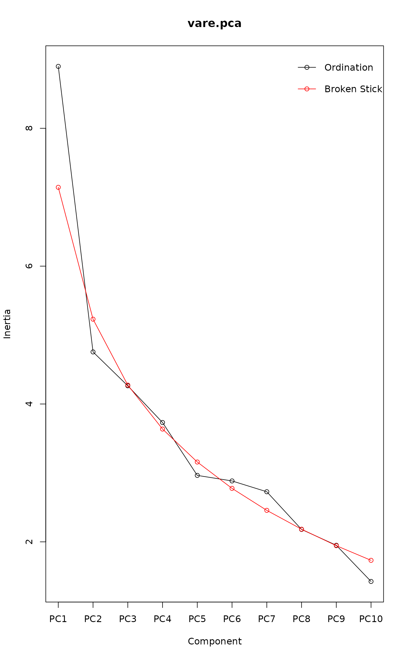
data(varespec)
vare.pca <- rda(varespec, scale = TRUE)
bstick(vare.pca)
#>       PC1       PC2       PC3       PC4       PC5       PC6       PC7       PC8 
#> 7.1438620 5.2308185 4.2742968 3.6366156 3.1583548 2.7757461 2.4569055 2.1836136 
#>       PC9      PC10      PC11      PC12      PC13      PC14      PC15      PC16 
#> 1.9444831 1.7319228 1.5406184 1.3667054 1.2072851 1.0601279 0.9234819 0.7959457 
#>      PC17      PC18      PC19      PC20      PC21      PC22      PC23 
#> 0.6763805 0.5638485 0.4575683 0.3568818 0.2612296 0.1701323 0.0831758 
screeplot(vare.pca, bstick = TRUE, type = "lines")