Tsallis Diversity and Corresponding Accumulation Curves

Function tsallis find Tsallis diversities with any scale or the corresponding evenness measures. Function tsallisaccum finds these statistics with accumulating sites.

tsallis(x, scales = seq(0, 2, 0.2), norm = FALSE, hill = FALSE)
tsallisaccum(x, scales = seq(0, 2, 0.2), permutations = 100, 
   raw = FALSE, subset, ...)
# S3 method for class 'tsallisaccum'
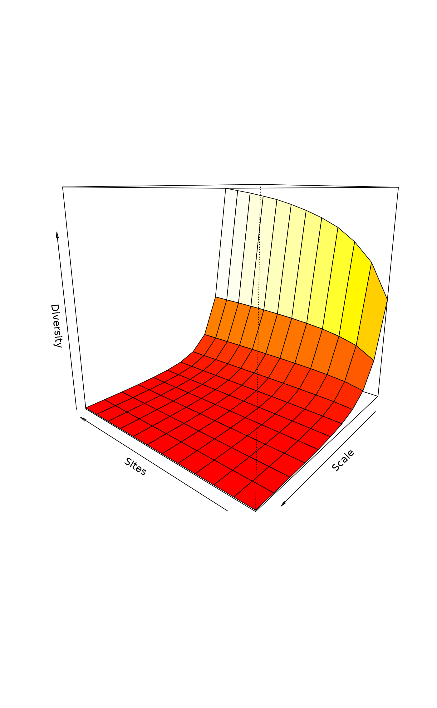
persp(x, theta = 220, phi = 15, col = heat.colors(100), zlim, ...)

Arguments

x

Community data matrix or plotting object.

scales

Scales of Tsallis diversity.

norm

Logical, if TRUE diversity values are normalized by their maximum (diversity value at equiprobability conditions).

hill

Calculate Hill numbers.

permutations

Usually an integer giving the number permutations, but can also be a list of control values for the permutations as returned by the function how, or a permutation matrix where each row gives the permuted indices.

raw

If FALSE then return summary statistics of permutations, and if TRUE then returns the individual permutations.

subset

logical expression indicating sites (rows) to keep: missing values are taken as FALSE.

theta, phi

angles defining the viewing direction. theta gives the azimuthal direction and phi the colatitude.

col

Colours used for surface.

zlim

Limits of vertical axis.

...

Other arguments which are passed to tsallis and to graphical functions.

Details

The Tsallis diversity (also equivalent to Patil and Taillie diversity) is a one-parametric generalised entropy function, defined as:

$$H_q = \frac{1}{q-1} (1-\sum_{i=1}^S p_i^q)$$

where \(q\) is a scale parameter, \(S\) the number of species in the sample (Tsallis 1988, Tothmeresz 1995). This diversity is concave for all \(q>0\), but non-additive (Keylock 2005). For \(q=0\) it gives the number of species minus one, as \(q\) tends to 1 this gives Shannon diversity, for \(q=2\) this gives the Simpson index (see function diversity).

If norm = TRUE, tsallis gives values normalized by the maximum:

$$H_q(max) = \frac{S^{1-q}-1}{1-q}$$

where \(S\) is the number of species. As \(q\) tends to 1, maximum is defined as \(ln(S)\).

If hill = TRUE, tsallis gives Hill numbers (numbers equivalents, see Jost 2007):

$$D_q = (1-(q-1) H)^{1/(1-q)}$$

Details on plotting methods and accumulating values can be found on the help pages of the functions renyi and renyiaccum.

Value

Function tsallis returns a data frame of selected indices. Function tsallisaccum with argument raw = FALSE returns a three-dimensional array, where the first dimension are the accumulated sites, second dimension are the diversity scales, and third dimension are the summary statistics mean, stdev, min, max, Qnt 0.025 and Qnt 0.975. With argument raw = TRUE the statistics on the third dimension are replaced with individual permutation results.

References

Tsallis, C. (1988) Possible generalization of Boltzmann-Gibbs statistics. J. Stat. Phis. 52, 479–487.

Tothmeresz, B. (1995) Comparison of different methods for diversity ordering. Journal of Vegetation Science 6, 283–290.

Patil, G. P. and Taillie, C. (1982) Diversity as a concept and its measurement. J. Am. Stat. Ass. 77, 548–567.

Keylock, C. J. (2005) Simpson diversity and the Shannon-Wiener index as special cases of a generalized entropy. Oikos 109, 203–207.

Jost, L (2007) Partitioning diversity into independent alpha and beta components. Ecology 88, 2427–2439.

Author

Péter Sólymos, solymos@ualberta.ca, based on the code of Roeland Kindt and Jari Oksanen written for renyi

See also

Plotting methods and accumulation routines are based on functions renyi and renyiaccum. An object of class tsallisaccum can be displayed with dynamic 3D function rgl.renyiaccum in the vegan3d package. See also settings for persp.

Examples

data(BCI)
i <- sample(nrow(BCI), 12)
x1 <- tsallis(BCI[i,])
x1
#>      0      0.2      0.4       0.6      0.8        1      1.2      1.4      1.6
#> 25 104 46.16214 22.10667 11.522497 6.562459 4.074718 2.736660 1.965873 1.492328
#> 36  91 40.76595 19.77916 10.481929 6.081803 3.846109 2.625076 1.910150 1.463936
#> 28  84 38.19298 18.72155  9.985457 5.818617 3.693896 2.532394 1.852192 1.427230
#> 45  80 35.98439 17.64135  9.493581 5.607534 3.609518 2.502487 1.844372 1.427545
#> 39  83 37.13183 17.98063  9.524369 5.542801 3.530494 2.435169 1.793695 1.391532
#> 24  94 42.55654 20.75558 10.992840 6.343926 3.979427 2.692702 1.944478 1.481404
#> 2   83 38.06254 18.90957 10.230614 6.028061 3.848471 2.638667 1.922477 1.472692
#> 47 101 44.24038 21.02130 10.943397 6.262025 3.920918 2.658316 1.925965 1.471937
#> 20  99 44.47873 21.56561 11.366723 6.530095 4.077327 2.746035 1.974163 1.498140
#> 38  81 36.25129 17.62089  9.387396 5.495029 3.516082 2.432141 1.793969 1.392413
#> 10  93 41.50369 20.10059 10.639881 6.164157 3.889803 2.648176 1.922207 1.470121
#> 8   87 39.98200 19.77567 10.603913 6.181934 3.908381 2.659907 1.928610 1.473408
#>         1.8         2
#> 25 1.183958 0.9726152
#> 36 1.169232 0.9648567
#> 28 1.145854 0.9499296
#> 45 1.148577 0.9528853
#> 39 1.123737 0.9360204
#> 24 1.178152 0.9694268
#> 2  1.174887 0.9683393
#> 47 1.173489 0.9672083
#> 20 1.187661 0.9748589
#> 38 1.124480 0.9365144
#> 10 1.172341 0.9663808
#> 8  1.173986 0.9671998
diversity(BCI[i,],"simpson") == x1[["2"]]
#>   25   36   28   45   39   24    2   47   20   38   10    8 
#> TRUE TRUE TRUE TRUE TRUE TRUE TRUE TRUE TRUE TRUE TRUE TRUE 
plot(x1)

x2 <- tsallis(BCI[i,],norm=TRUE)
x2
#>    0       0.2       0.4       0.6       0.8         1       1.2       1.4
#> 25 1 0.9142073 0.8658106 0.8481902 0.8541991 0.8755378 0.9035478 0.9310603
#> 36 1 0.8998669 0.8431295 0.8216927 0.8272622 0.8505725 0.8820846 0.9137994
#> 28 1 0.8997942 0.8397547 0.8130733 0.8129096 0.8314621 0.8602754 0.8916927
#> 45 1 0.8821127 0.8163126 0.7912066 0.7963976 0.8213811 0.8559075 0.8914611
#> 39 1 0.8833633 0.8127010 0.7799621 0.7774979 0.7968043 0.8286189 0.8643658
#> 24 1 0.9149445 0.8667059 0.8486326 0.8536824 0.8738548 0.9008891 0.9279024
#> 2  1 0.9055048 0.8546877 0.8377974 0.8455660 0.8685692 0.8978637 0.9264249
#> 47 1 0.8972246 0.8387068 0.8167095 0.8229465 0.8477709 0.8810155 0.9141216
#> 20 1 0.9168340 0.8714005 0.8563191 0.8638340 0.8853802 0.9124664 0.9383899
#> 38 1 0.8797117 0.8089277 0.7777332 0.7771539 0.7978912 0.8304023 0.8662156
#> 10 1 0.9001004 0.8450759 0.8255446 0.8324355 0.8561634 0.8872568 0.9180261
#> 8  1 0.9154260 0.8674322 0.8491531 0.8535754 0.8729254 0.8992501 0.9258854
#>          1.6       1.8         2
#> 25 0.9538440 0.9706141 0.9819673
#> 36 0.9407648 0.9611954 0.9754595
#> 28 0.9203563 0.9436787 0.9612382
#> 45 0.9225835 0.9470176 0.9647964
#> 39 0.8978144 0.9257229 0.9472977
#> 24 0.9507028 0.9678509 0.9797399
#> 2  0.9501791 0.9678597 0.9800060
#> 47 0.9418898 0.9625904 0.9767846
#> 20 0.9594192 0.9746101 0.9847059
#> 38 0.8993700 0.9268720 0.9480763
#> 10 0.9438798 0.9632975 0.9767719
#> 8  0.9486740 0.9660687 0.9783170
plot(x2)

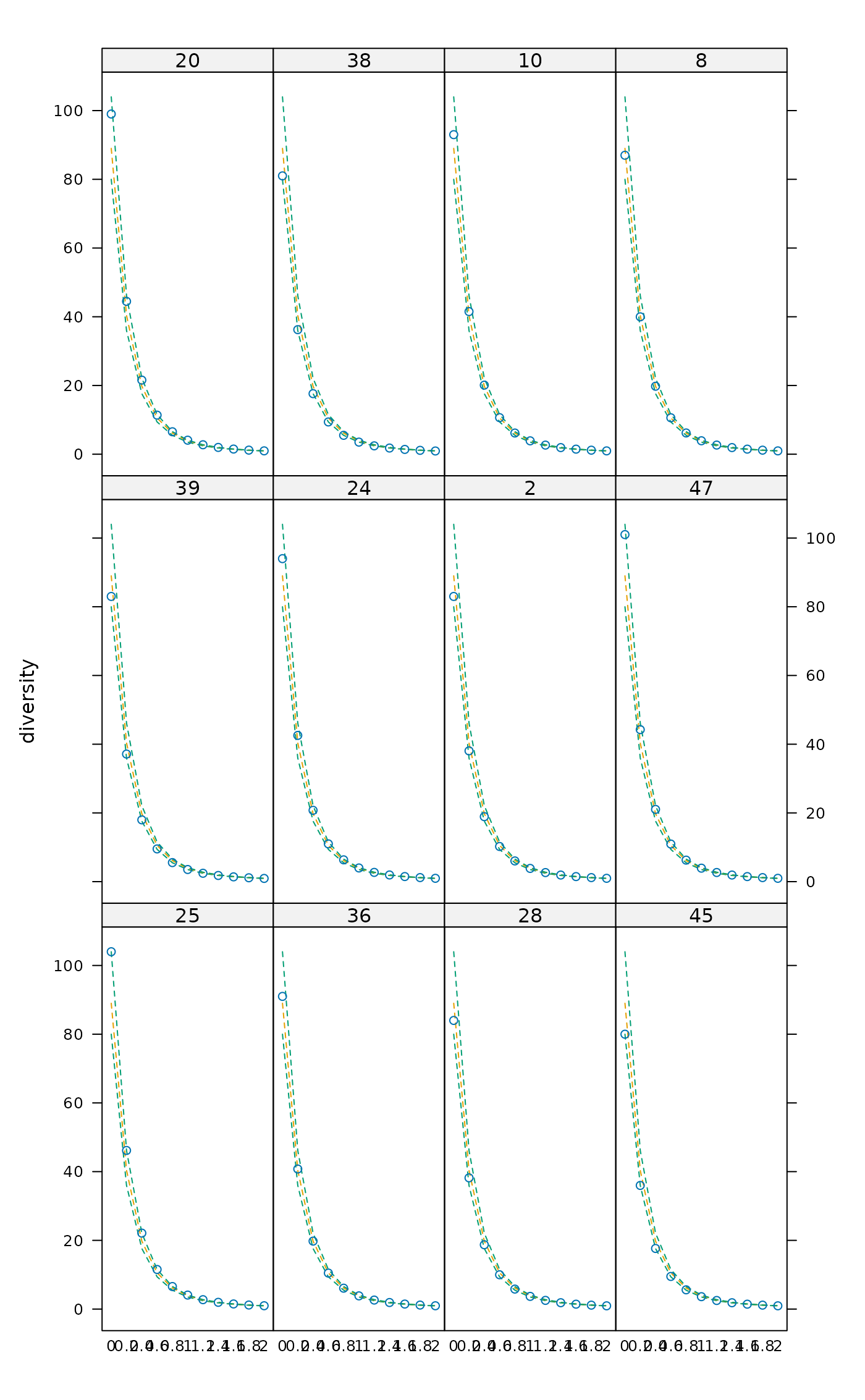
mod1 <- tsallisaccum(BCI[i,])
plot(mod1, as.table=TRUE, col = c(1, 2, 2))

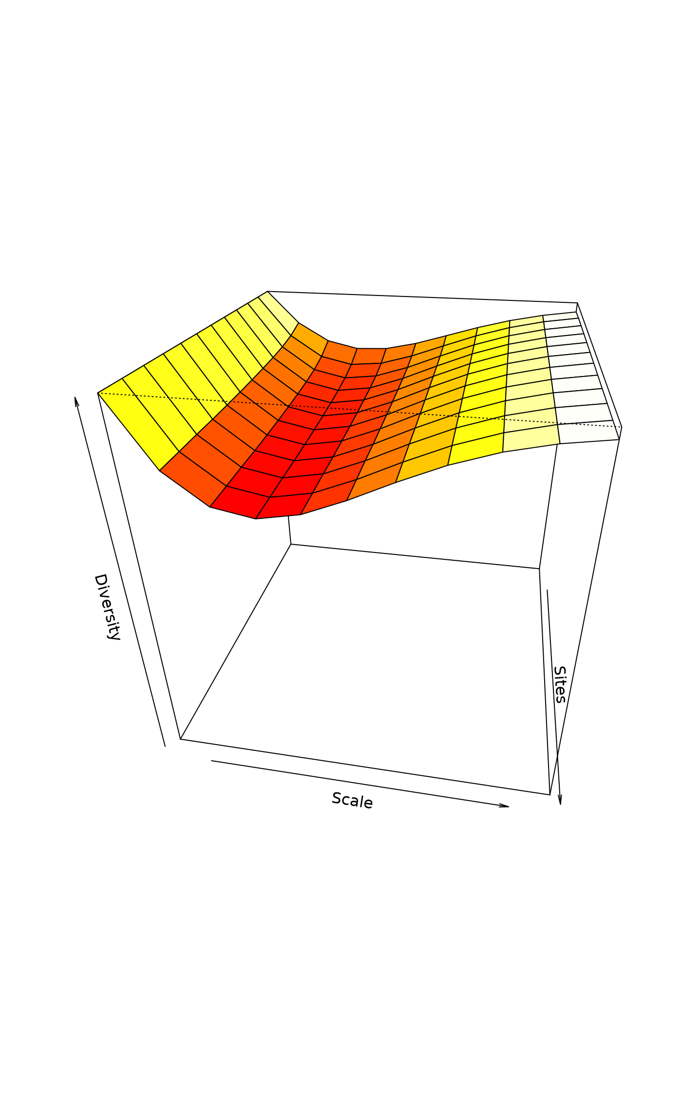
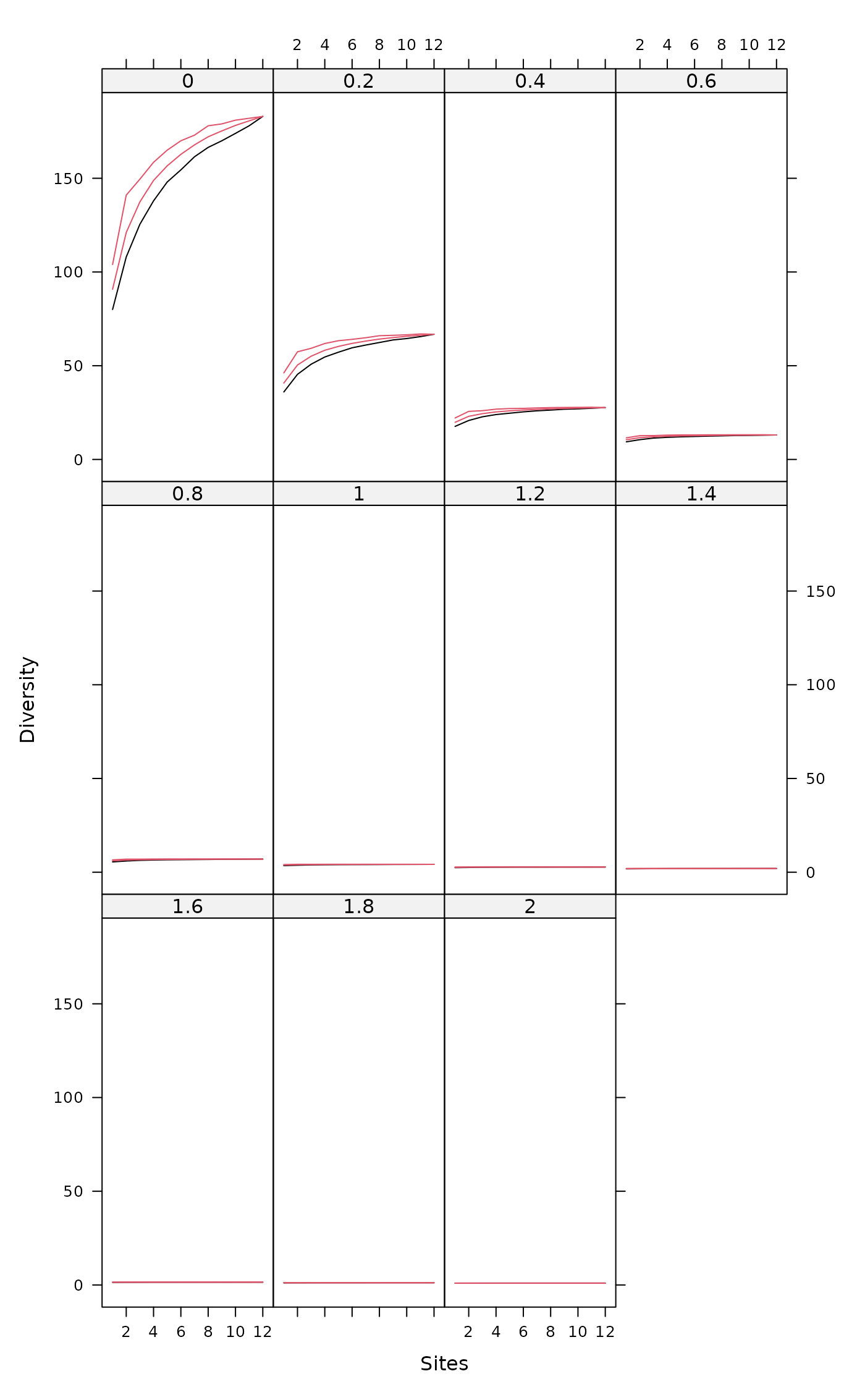persp(mod1)

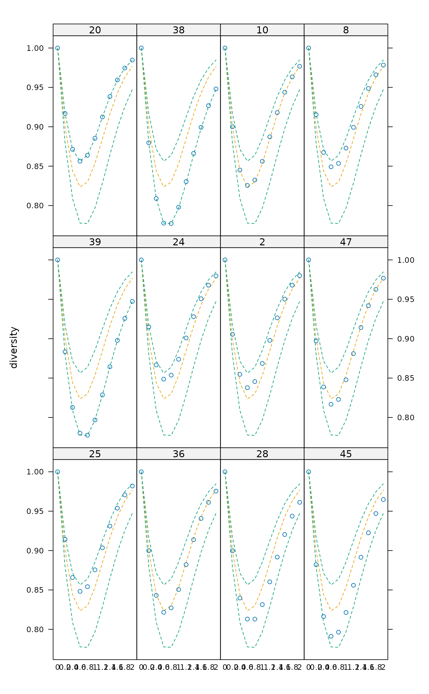
mod2 <- tsallisaccum(BCI[i,], norm=TRUE)
persp(mod2,theta=100,phi=30)