Functional Diversity and Community Distances from Species Trees

Functional diversity is defined as the total branch length in a trait dendrogram connecting all species, but excluding the unnecessary root segments of the tree (Petchey and Gaston 2006). Tree distance is the increase in total branch length when combining two sites.

treedive(comm, tree, match.force = TRUE, verbose = TRUE)
treeheight(tree)
treedist(x, tree, relative = TRUE, match.force = TRUE, ...)

Arguments

comm, x: Community data frame or matrix.
tree: A dendrogram which for treedive must be for species (columns).
match.force: Force matching of column names in data (comm, x) and labels in tree. If FALSE, matching only happens when dimensions differ (with a warning or message). The order of data must match to the order in tree if matching by names is not done.
verbose: Print diagnostic messages and warnings.
relative: Use distances relative to the height of combined tree.
...: Other arguments passed to functions (ignored).

Details

Function treeheight finds the sum of lengths of connecting segments in a dendrogram produced by hclust, or other dendrogram that can be coerced to a correct type using as.hclust. When applied to a clustering of species traits, this is a measure of functional diversity (Petchey and Gaston 2002, 2006), and when applied to phylogenetic trees this is phylogenetic diversity.

Function treedive finds the treeheight for each site (row) of a community matrix. The function uses a subset of dendrogram for those species that occur in each site, and excludes the tree root if that is not needed to connect the species (Petchey and Gaston 2006). The subset of the dendrogram is found by first calculating cophenetic distances from the input dendrogram, then reconstructing the dendrogram for the subset of the cophenetic distance matrix for species occurring in each site. Diversity is 0 for one species, and NA for empty communities.

Function treedist finds the dissimilarities among trees. Pairwise dissimilarity of two trees is found by combining species in a common tree and seeing how much of the tree height is shared and how much is unique. With relative = FALSE the dissimilarity is defined as \(2 (A \cup B) - A - B\), where \(A\) and \(B\) are heights of component trees and \(A \cup B\) is the height of the combined tree. With relative = TRUE the dissimilarity is \((2(A \cup B)-A-B)/(A \cup B)\). Although the latter formula is similar to Jaccard dissimilarity (see vegdist, designdist), it is not in the range \(0 \ldots 1\), since combined tree can add a new root. When two zero-height trees are combined into a tree of above zero height, the relative index attains its maximum value \(2\). The dissimilarity is zero from a combined zero-height tree.

The functions need a dendrogram of species traits or phylogenies as an input. If species traits contain factor or ordered factor variables, it is recommended to use Gower distances for mixed data (function daisy in package cluster), and usually the recommended clustering method is UPGMA (method = "average" in function hclust) (Podani and Schmera 2006). Phylogenetic trees can be changed into dendrograms using function as.hclust.phylo in the ape package.

It is possible to analyse the non-randomness of tree diversity using oecosimu. This needs specifying an adequate Null model, and the results will change with this choice.

Value

A vector of diversity values or a single tree height, or a dissimilarity structure that inherits from dist and can be used similarly.

References

Lozupone, C. and Knight, R. 2005. UniFrac: a new phylogenetic method for comparing microbial communities. Applied and Environmental Microbiology 71, 8228–8235.

Petchey, O.L. and Gaston, K.J. 2002. Functional diversity (FD), species richness and community composition. Ecology Letters 5, 402–411.

Petchey, O.L. and Gaston, K.J. 2006. Functional diversity: back to basics and looking forward. Ecology Letters 9, 741–758.

Podani J. and Schmera, D. 2006. On dendrogram-based methods of functional diversity. Oikos 115, 179–185.

Author

Jari Oksanen

Examples


## There is no data set on species properties yet, and we demonstrate
## the methods using phylogenetic trees
data(dune)
data(dune.phylodis)
cl <- hclust(dune.phylodis)
treedive(dune, cl)
#> forced matching of 'tree' labels and 'comm' names
#>         1         2         3         4         5         6         7         8 
#>  384.0913  568.8791 1172.9455 1327.9317 1426.9067 1391.1628 1479.5062 1523.0792 
#>         9        10        11        12        13        14        15        16 
#> 1460.0423 1316.4832 1366.9960 1423.5582  895.1120 1457.2705 1505.9501 1187.5165 
#>        17        18        19        20 
#>  517.6920 1394.5162 1470.4671 1439.5571 
## Significance test using Null model communities.
## The current choice fixes numbers of species and picks species
## proportionally to their overall frequency
oecosimu(dune, treedive, "r1", tree = cl, verbose = FALSE)
#> Warning: nullmodel transformed 'comm' to binary data
#> oecosimu object
#> 
#> Call: oecosimu(comm = dune, nestfun = treedive, method = "r1", tree =
#> cl, verbose = FALSE)
#> 
#> nullmodel method ‘r1’ with 99 simulations
#> 
#> alternative hypothesis: statistic is less or greater than simulated values
#> 
#>    statistic       SES    mean    2.5%     50%  97.5% Pr(sim.)   
#> 1     384.09 -1.206187  702.95  384.59  608.23 1232.0     0.07 . 
#> 2     568.88 -2.609672 1237.84  760.64 1312.03 1568.2     0.01 **
#> 3    1172.95 -0.098178 1201.99  630.08 1330.77 1539.4     0.63   
#> 4    1327.93 -0.314810 1402.52  837.21 1469.98 1723.5     0.45   
#> 5    1426.91 -0.194760 1471.99  892.81 1523.66 1769.1     0.39   
#> 6    1391.16  0.201881 1339.46  737.03 1428.21 1600.7     0.71   
#> 7    1479.51  0.215783 1429.66  816.92 1483.05 1717.9     0.93   
#> 8    1523.08  0.640121 1352.61  809.16 1439.33 1711.7     0.51   
#> 9    1460.04  0.017371 1455.99  866.56 1526.62 1745.6     0.63   
#> 10   1316.48 -0.184064 1364.90  726.04 1444.71 1694.8     0.51   
#> 11   1367.00  0.772702 1144.00  653.11 1252.77 1528.0     0.53   
#> 12   1423.56  0.955266 1140.46  612.92 1272.20 1542.2     0.29   
#> 13    895.11 -0.925085 1172.53  647.30 1264.01 1580.7     0.53   
#> 14   1457.27  1.604499  956.83  506.41  884.44 1403.6     0.01 **
#> 15   1505.95  1.448057 1049.20  579.92 1211.83 1427.4     0.03 * 
#> 16   1187.52  0.346202 1078.28  539.47 1236.78 1475.6     0.83   
#> 17    517.69 -1.559525  985.09  508.62 1127.17 1392.0     0.09 . 
#> 18   1394.52  0.777739 1168.57  604.63 1286.03 1515.0     0.39   
#> 19   1470.47  0.996512 1180.17  605.56 1287.32 1495.7     0.17   
#> 20   1439.56  1.268059 1045.53  527.95 1170.61 1446.1     0.07 . 
#> ---
#> Signif. codes:  0 ‘***’ 0.001 ‘**’ 0.01 ‘*’ 0.05 ‘.’ 0.1 ‘ ’ 1
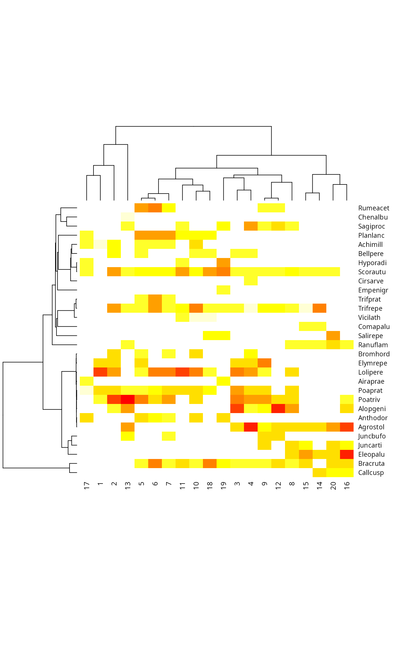
## Phylogenetically ordered community table
dtree <- treedist(dune, cl)
tabasco(dune, hclust(dtree), cl)

## Use tree distances in distance-based RDA
dbrda(dtree ~ 1)
#> 
#> Call: dbrda(formula = dtree ~ 1)
#> 
#>               Inertia Rank RealDims
#> Total           2.183              
#> Unconstrained   2.183   19       10
#> 
#> Inertia is squared Treedist distance
#> 
#> Eigenvalues for unconstrained axes:
#>   MDS1   MDS2   MDS3   MDS4   MDS5   MDS6   MDS7   MDS8 
#> 1.1971 0.4546 0.2967 0.1346 0.1067 0.0912 0.0391 0.0190 
#> (Showing 8 of 19 unconstrained eigenvalues)
#>