Additive Regression and Transformations using ace or avas
transace.Rdtransace is ace packaged for easily automatically
transforming all variables in a formula without a left-hand side.
transace is a fast
one-iteration version of transcan without imputation of
NAs. The ggplot method makes nice transformation plots
using ggplot2. Binary variables are automatically kept linear,
and character or factor variables are automatically treated as categorical.
areg.boot uses areg or
avas to fit additive regression models allowing
all variables in the model (including the left-hand-side) to be
transformed, with transformations chosen so as to optimize certain
criteria. The default method uses areg whose goal it is
to maximize \(R^2\). method="avas" explicity tries to
transform the response variable so as to stabilize the variance of the
residuals. All-variables-transformed models tend to inflate R^2
and it can be difficult to get confidence limits for each
transformation. areg.boot solves both of these problems using
the bootstrap. As with the validate function in the
rms library, the Efron bootstrap is used to estimate the
optimism in the apparent \(R^2\), and this optimism is subtracted
from the apparent \(R^2\) to optain a bias-corrected \(R^2\).
This is done however on the transformed response variable scale.
Tests with 3 predictors show that the avas and
ace estimates are unstable unless the sample size
exceeds 350. Apparent \(R^2\) with low sample sizes can be very
inflated, and bootstrap estimates of \(R^2\) can be even more
unstable in such cases, resulting in optimism-corrected \(R^2\) that
are much lower even than the actual \(R^2\). The situation can be
improved a little by restricting predictor transformations to be
monotonic. On the other hand, the areg approach allows one to
control overfitting by specifying the number of knots to use for each
continuous variable in a restricted cubic spline function.
For method="avas" the response transformation is restricted to
be monotonic. You can specify restrictions for transformations of
predictors (and linearity for the response). When the first argument
is a formula, the function automatically determines which variables
are categorical (i.e., factor, category, or character
vectors). Specify linear transformations by enclosing variables by
the identify function (I()), and specify monotonicity by using
monotone(variable). Monotonicity restrictions are not
allowed with method="areg".
The summary method for areg.boot computes
bootstrap estimates of standard errors of differences in predicted
responses (usually on the original scale) for selected levels of each
predictor against the lowest level of the predictor. The smearing
estimator (see below) can be used here to estimate differences in
predicted means, medians, or many other statistics. By default,
quartiles are used for continuous predictors and all levels are used
for categorical ones. See Details below. There is also a
plot method for plotting transformation estimates,
transformations for individual bootstrap re-samples, and pointwise
confidence limits for transformations. Unless you already have a
par(mfrow=) in effect with more than one row or column,
plot will try to fit the plots on one page. A
predict method computes predicted values on the original
or transformed response scale, or a matrix of transformed
predictors. There is a Function method for producing a
list of R functions that perform the final fitted transformations.
There is also a print method for areg.boot
objects.
When estimated means (or medians or other statistical parameters) are
requested for models fitted with areg.boot (by
summary.areg.boot or predict.areg.boot), the
“smearing” estimator of Duan (1983) is used. Here we
estimate the mean of the untransformed response by computing the
arithmetic mean of \(ginverse(lp + residuals)\),
where ginverse is the inverse of the nonparametric
transformation of the response (obtained by reverse linear
interpolation), lp is the linear predictor for an individual
observation on the transformed scale, and residuals is the
entire vector of residuals estimated from the fitted model, on the
transformed scales (n residuals for n original observations). The
smearingEst function computes the general smearing estimate.
For efficiency smearingEst recognizes that quantiles are
transformation-preserving, i.e., when one wishes to estimate a
quantile of the untransformed distribution one just needs to compute
the inverse transformation of the transformed estimate after the
chosen quantile of the vector of residuals is added to it. When the
median is desired, the estimate is
\(ginverse(lp + \mbox{median}(residuals))\).
See the last example for how smearingEst can be used outside of
areg.boot.
Mean is a generic function that returns an R function to
compute the estimate of the mean of a variable. Its input is
typically some kind of model fit object. Likewise, Quantile is
a generic quantile function-producing function. Mean.areg.boot
and Quantile.areg.boot create functions of a vector of linear
predictors that transform them into the smearing estimates of the mean
or quantile of the response variable,
respectively. Quantile.areg.boot produces exactly the same
value as predict.areg.boot or smearingEst. Mean
approximates the mapping of linear predictors to means over an evenly
spaced grid of by default 200 points. Linear interpolation is used
between these points. This approximate method is much faster than the
full smearing estimator once Mean creates the function. These
functions are especially useful in nomogram (see the
example on hypothetical data).
transace(formula, trim=0.01, data=environment(formula))

# S3 method for class 'transace'
print(x, ...)

# S3 method for class 'transace'
ggplot(data, mapping, ..., environment, nrow=NULL)

areg.boot(x, data, weights, subset, na.action=na.delete,
          B=100, method=c("areg","avas"), nk=4, evaluation=100, valrsq=TRUE,
          probs=c(.25,.5,.75), tolerance=NULL)

# S3 method for class 'areg.boot'
print(x, ...)

# S3 method for class 'areg.boot'
plot(x, ylim, boot=TRUE, col.boot=2, lwd.boot=.15,
     conf.int=.95, ...)

smearingEst(transEst, inverseTrans, res,
            statistic=c('median','quantile','mean','fitted','lp'),
            q)

# S3 method for class 'areg.boot'
summary(object, conf.int=.95, values, adj.to,
        statistic='median', q, ...)

# S3 method for class 'summary.areg.boot'
print(x, ...)

# S3 method for class 'areg.boot'
predict(object, newdata,
        statistic=c("lp", "median",
                    "quantile", "mean", "fitted", "terms"),
        q=NULL, ...)

# S3 method for class 'areg.boot'
Function(object, type=c('list','individual'),
         ytype=c('transformed','inverse'),
         prefix='.', suffix='', pos=-1, ...)

Mean(object, ...)

Quantile(object, ...)

# S3 method for class 'areg.boot'
Mean(object, evaluation=200, ...)

# S3 method for class 'areg.boot'
Quantile(object, q=.5, ...)
Arguments
- formula
a formula without a left-hand-side variable. Variables may be enclosed in
monotone(), linear(), categorical()to make certain assumptions about transformations.categoricalandlinearneed not be specified if they can be summized from the variable values.- x
for
areg.bootxis a formula. Forprintorplot, an object created byareg.bootortransace. Forprint.summary.areg.boot, and object created bysummary.areg.boot. Forggplotis the result oftransace.- object
an object created by
areg.boot, or a model fit object suitable forMeanorQuantile.- transEst
a vector of transformed values. In log-normal regression these could be predicted log(Y) for example.
- inverseTrans
a function specifying the inverse transformation needed to change
transEstto the original untransformed scale.inverseTransmay also be a 2-element list defining a mapping from the transformed values to untransformed values. Linear interpolation is used in this case to obtain untransform values.- trim
quantile to which to trim original and transformed values for continuous variables for purposes of plotting the transformations with
ggplot.transace- nrow
the number of rows to graph for
transacetransformations, with the default chosen byggplot2- data
data frame to use if
xis a formula and variables are not already in the search list. Forggplotis atransaceobject.- environment,mapping
ignored
- weights
a numeric vector of observation weights. By default, all observations are weighted equally.
- subset
an expression to subset data if
xis a formula- na.action
a function specifying how to handle
NAs. Default isna.delete.- B
number of bootstrap samples (default=100)
- method
"areg"(the default) or"avas"- nk
number of knots for continuous variables not restricted to be linear. Default is 4. One or two is not allowed.
nk=0forces linearity for all continuous variables.- evaluation
number of equally-spaced points at which to evaluate (and save) the nonparametric transformations derived by
avasorace. Default is 100. ForMean.areg.boot,evaluationis the number of points at which to evaluate exact smearing estimates, to approximate them using linear interpolation (default is 200).- valrsq
set to
TRUEto more quickly do bootstrapping without validating \(R^2\)- probs
vector probabilities denoting the quantiles of continuous predictors to use in estimating effects of those predictors
- tolerance
singularity criterion; list source code for the
lm.fit.qr.barefunction.- res
a vector of residuals from the transformed model. Not required when
statistic="lp"orstatistic="fitted".- statistic
statistic to estimate with the smearing estimator. For
smearingEst, the default results in computation of the sample median of the model residuals, thensmearingEstadds the median residual and back-transforms to get estimated median responses on the original scale.statistic="lp"causes predicted transformed responses to be computed. ForsmearingEst, the result (forstatistic="lp") is the input argumenttransEst.statistic="fitted"gives predicted untransformed responses, i.e., \(ginverse(lp)\), where ginverse is the inverse of the estimated response transformation, estimated by reverse linear interpolation on the tabulated nonparametric response transformation or by using an explicit analytic function.statistic="quantile"generalizes"median"to any single quantileqwhich must be specified."mean"causes the population mean response to be estimated. Forpredict.areg.boot,statistic="terms"returns a matrix of transformed predictors.statisticcan also be any R function that computes a single value on a vector of values, such asstatistic=var. Note that in this case the function name is not quoted.- q
a single quantile of the original response scale to estimate, when
statistic="quantile", or forQuantile.areg.boot.- ylim
2-vector of y-axis limits
- boot
set to
FALSEto not plot any bootstrapped transformations. Set it to an integer k to plot the first k bootstrap estimates.- col.boot
color for bootstrapped transformations
- lwd.boot
line width for bootstrapped transformations
- conf.int
confidence level (0-1) for pointwise bootstrap confidence limits and for estimated effects of predictors in
summary.areg.boot. The latter assumes normality of the estimated effects.- values
a list of vectors of settings of the predictors, for predictors for which you want to overide settings determined from
probs. The list must have named components, with names corresponding to the predictors. Example:values=list(x1=c(2,4,6,8), x2=c(-1,0,1))specifies thatsummaryis to estimate the effect onyof changingx1from 2 to 4, 2 to 6, 2 to 8, and separately, of changingx2from -1 to 0 and -1 to 1.- adj.to
a named vector of adjustment constants, for setting all other predictors when examining the effect of a single predictor in
summary. The more nonlinear is the transformation ofythe more the adjustment settings will matter. Default values are the medians of the values defined byvaluesorprobs. You only need to name the predictors for which you are overriding the default settings. Example:adj.to=c(x2=0,x5=10)will setx2to 0 andx5to 10 when assessing the impact of variation in the other predictors.- newdata
a data frame or list containing the same number of values of all of the predictors used in the fit. For
factorpredictors the levels attribute do not need to be in the same order as those used in the original fit, and not all levels need to be represented. Ifnewdatais omitted, you can still obtain linear predictors (on the transformed response scale) and fitted values (on the original response scale), but not"terms".- type
specifies how
Functionis to return the series of functions that define the transformations of all variables. By default a list is created, with the names of the list elements being the names of the variables. Specifytype="individual"to have separate functions created in the current environment (pos=-1, the default) or in location defined byposifwhereis specified. For the latter method, the names of the objects created are the names of the corresponding variables, prefixed byprefixand withsuffixappended to the end. If any ofpos,prefix, orsuffixis specified,typeis automatically set to"individual".- ytype
By default the first function created by
Functionis the y-transformation. Specifyytype="inverse"to instead create the inverse of the transformation, to be able to obtain originally scaled y-values.- prefix
character string defining the prefix for function names created when
type="individual". By default, the function specifying the transformation for variablexwill be named.x.- suffix
character string defining the suffix for the function names
- pos
See
assign.- ...
arguments passed to other functions. Ignored for
print.transaceandggplot.transace.
Value
transace returns a list of class transace containing
these elements: n (number of non-missing observations used), transformed (a matrix containing transformed values), rsq (vector of \(R^2\) with which each
variable can be predicted from the others), omitted (row
numbers of data that were deleted due to NAs),
trantab (compact transformation lookups), levels
(original levels of character and factor varibles if the input was a
data frame), trim (value of trim passed to
transace), limits (the limits for plotting raw and
transformed variables, computed from trim), and type (a
vector of transformation types used for the variables).
areg.boot returns a list of class areg.boot containing
many elements, including (if valrsq is TRUE)
rsquare.app and rsquare.val. summary.areg.boot
returns a list of class summary.areg.boot containing a matrix
of results for each predictor and a vector of adjust-to settings. It
also contains the call and a label for the statistic that was
computed. A print method for these objects handles the
printing. predict.areg.boot returns a vector unless
statistic="terms", in which case it returns a
matrix. Function.areg.boot returns by default a list of
functions whose argument is one of the variables (on the original
scale) and whose returned values are the corresponding transformed
values. The names of the list of functions correspond to the names of
the original variables. When type="individual",
Function.areg.boot invisibly returns the vector of names of the
created function objects. Mean.areg.boot and
Quantile.areg.boot also return functions.
smearingEst returns a vector of estimates of distribution
parameters of class labelled so that print.labelled wil
print a label documenting the estimate that was used (see
label). This label can be retrieved for other purposes
by using e.g. label(obj), where obj was the vector
returned by smearingEst.
Details
As transace only does one iteration over the predictors, it may
not find optimal transformations and it will be dependent on the order
of the predictors in x.
ace and avas standardize transformed variables to have
mean zero and variance one for each bootstrap sample, so if a
predictor is not important it will still consistently have a positive
regression coefficient. Therefore using the bootstrap to estimate
standard errors of the additive least squares regression coefficients
would not help in drawing inferences about the importance of the
predictors. To do this, summary.areg.boot computes estimates
of, e.g., the inter-quartile range effects of predictors in predicting
the response variable (after untransforming it). As an example, at
each bootstrap repetition the estimated transformed value of one of
the predictors is computed at the lower quartile, median, and upper
quartile of the raw value of the predictor. These transformed x
values are then multipled by the least squares estimate of the partial
regression coefficient for that transformed predictor in predicting
transformed y. Then these weighted transformed x values have the
weighted transformed x value corresponding to the lower quartile
subtracted from them, to estimate an x effect accounting for
nonlinearity. The last difference computed is then the standardized
effect of raising x from its lowest to its highest quartile. Before
computing differences, predicted values are back-transformed to be on
the original y scale in a way depending on statistic and
q. The sample standard deviation of these effects (differences)
is taken over the bootstrap samples, and this is used to compute
approximate confidence intervals for effects andapproximate P-values,
both assuming normality.
predict does not re-insert NAs corresponding to
observations that were dropped before the fit, when newdata is
omitted.
statistic="fitted" estimates the same quantity as
statistic="median" if the residuals on the transformed response
have a symmetric distribution. The two provide identical estimates
when the sample median of the residuals is exactly zero. The sample
mean of the residuals is constrained to be exactly zero although this
does not simplify anything.
References
Harrell FE, Lee KL, Mark DB (1996): Stat in Med 15:361–387.
Duan N (1983): Smearing estimate: A nonparametric retransformation method. JASA 78:605–610.
Wang N, Ruppert D (1995): Nonparametric estimation of the transformation in the transform-both-sides regression model. JASA 90:522–534.
Examples
# xtrans <- transace(~ monotone(age) + sex + blood.pressure + categorical(race.code))
# print(xtrans) # show R^2s and a few other things
# ggplot(xtrans) # show transformations
# Generate random data from the model y = exp(x1 + epsilon/3) where
# x1 and epsilon are Gaussian(0,1)
set.seed(171) # to be able to reproduce example
x1 <- rnorm(200)
x2 <- runif(200) # a variable that is really unrelated to y]
x3 <- factor(sample(c('cat','dog','cow'), 200,TRUE)) # also unrelated to y
y <- exp(x1 + rnorm(200)/3)
f <- areg.boot(y ~ x1 + x2 + x3, B=40)
#> 1
2
3
4
5
6
7
8
9
10
11
12
13
14
15
16
17
18
19
20
21
22
23
24
25
26
27
28
29
30
31
32
33
34
35
36
37
38
39
40
f
#>
#> areg Additive Regression Model
#>
#> areg.boot(x = y ~ x1 + x2 + x3, B = 40)
#>
#>
#> Predictor Types
#>
#> type d.f.
#> x1 s 3
#> x2 s 3
#> x3 c 2
#>
#> y type: s d.f.: 3
#>
#> n= 200 p= 3
#>
#> Apparent R2 on transformed Y scale: 0.905
#> Bootstrap validated R2 : 0.862
#>
#> Coefficients of standardized transformations:
#>
#> Intercept x1 x2 x3
#> 1.25e-16 9.51e-01 9.51e-01 9.51e-01
#>
#>
#> Residuals on transformed scale:
#>
#> Min 1Q Median 3Q Max Mean S.D.
#> -7.12e-01 -2.08e-01 -7.07e-03 1.70e-01 9.52e-01 -4.49e-18 3.09e-01
#>
plot(f)
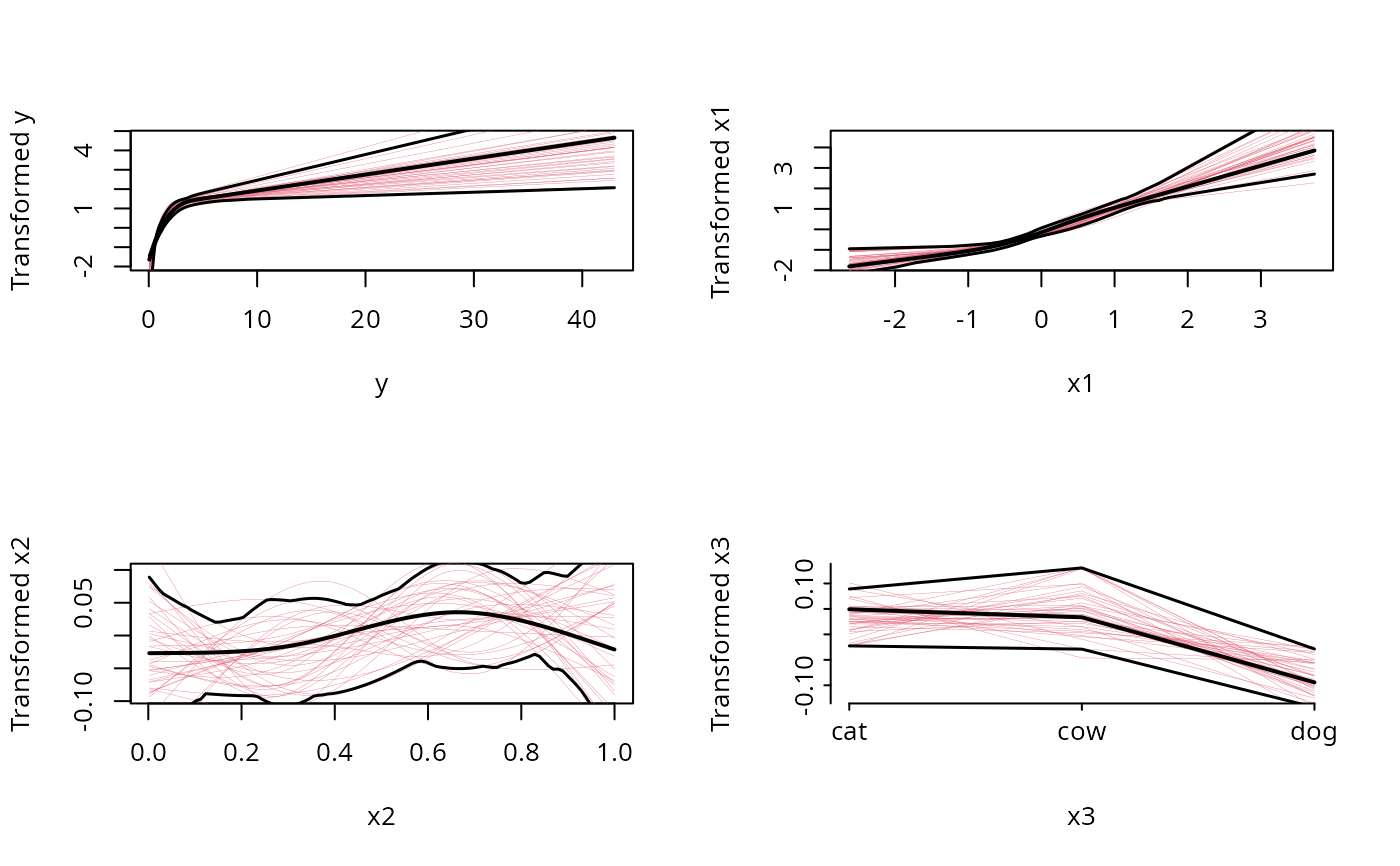 # Note that the fitted transformation of y is very nearly log(y)
# (the appropriate one), the transformation of x1 is nearly linear,
# and the transformations of x2 and x3 are essentially flat
# (specifying monotone(x2) if method='avas' would have resulted
# in a smaller confidence band for x2)
summary(f)
#> summary.areg.boot(object = f)
#>
#> Estimates based on 40 resamples
#>
#>
#>
#> Values to which predictors are set when estimating
#> effects of other predictors:
#>
#> y x1 x2 x3
#> 1.0004 0.0528 0.5117 2.0000
#>
#> Estimates of differences of effects on Median Y (from first X
#> value), and bootstrap standard errors of these differences.
#> Settings for X are shown as row headings.
#>
#>
#> Predictor: x1
#>
#> x Differences S.E Lower 0.95 Upper 0.95 Z Pr(|Z|)
#> -0.6289 0.000 NA NA NA NA NA
#> 0.0528 0.511 0.0453 0.422 0.60 11.3 1.49e-29
#> 0.6979 1.400 0.1282 1.148 1.65 10.9 9.75e-28
#>
#>
#> Predictor: x2
#>
#> x Differences S.E Lower 0.95 Upper 0.95 Z Pr(|Z|)
#> 0.223 0.0000 NA NA NA NA NA
#> 0.512 0.0362 0.0435 -0.0491 0.121 0.832 0.405
#> 0.768 0.0427 0.0699 -0.0942 0.180 0.612 0.541
#>
#>
#> Predictor: x3
#>
#> x Differences S.E Lower 0.95 Upper 0.95 Z Pr(|Z|)
#> cat 0.0000 NA NA NA NA NA
#> cow -0.0135 0.0605 -0.132 0.1050 -0.223 0.82357
#> dog -0.1184 0.0409 -0.198 -0.0383 -2.898 0.00376
# use summary(f, values=list(x2=c(.2,.5,.8))) for example if you
# want to use nice round values for judging effects
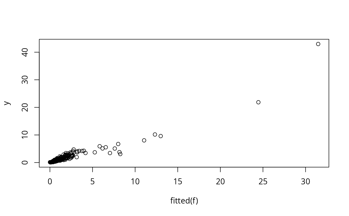
# Plot Y hat vs. Y (this doesn't work if there were NAs)
plot(fitted(f), y) # or: plot(predict(f,statistic='fitted'), y)
# Note that the fitted transformation of y is very nearly log(y)
# (the appropriate one), the transformation of x1 is nearly linear,
# and the transformations of x2 and x3 are essentially flat
# (specifying monotone(x2) if method='avas' would have resulted
# in a smaller confidence band for x2)
summary(f)
#> summary.areg.boot(object = f)
#>
#> Estimates based on 40 resamples
#>
#>
#>
#> Values to which predictors are set when estimating
#> effects of other predictors:
#>
#> y x1 x2 x3
#> 1.0004 0.0528 0.5117 2.0000
#>
#> Estimates of differences of effects on Median Y (from first X
#> value), and bootstrap standard errors of these differences.
#> Settings for X are shown as row headings.
#>
#>
#> Predictor: x1
#>
#> x Differences S.E Lower 0.95 Upper 0.95 Z Pr(|Z|)
#> -0.6289 0.000 NA NA NA NA NA
#> 0.0528 0.511 0.0453 0.422 0.60 11.3 1.49e-29
#> 0.6979 1.400 0.1282 1.148 1.65 10.9 9.75e-28
#>
#>
#> Predictor: x2
#>
#> x Differences S.E Lower 0.95 Upper 0.95 Z Pr(|Z|)
#> 0.223 0.0000 NA NA NA NA NA
#> 0.512 0.0362 0.0435 -0.0491 0.121 0.832 0.405
#> 0.768 0.0427 0.0699 -0.0942 0.180 0.612 0.541
#>
#>
#> Predictor: x3
#>
#> x Differences S.E Lower 0.95 Upper 0.95 Z Pr(|Z|)
#> cat 0.0000 NA NA NA NA NA
#> cow -0.0135 0.0605 -0.132 0.1050 -0.223 0.82357
#> dog -0.1184 0.0409 -0.198 -0.0383 -2.898 0.00376
# use summary(f, values=list(x2=c(.2,.5,.8))) for example if you
# want to use nice round values for judging effects
# Plot Y hat vs. Y (this doesn't work if there were NAs)
plot(fitted(f), y) # or: plot(predict(f,statistic='fitted'), y)
 # Show fit of model by varying x1 on the x-axis and creating separate
# panels for x2 and x3. For x2 using only a few discrete values
newdat <- expand.grid(x1=seq(-2,2,length=100),x2=c(.25,.75),
x3=c('cat','dog','cow'))
yhat <- predict(f, newdat, statistic='fitted')
# statistic='mean' to get estimated mean rather than simple inverse trans.
xYplot(yhat ~ x1 | x2, groups=x3, type='l', data=newdat)
#> Error in eval(parse(text = yvname), data): object 'yhat' not found
if (FALSE) { # \dontrun{
# Another example, on hypothetical data
f <- areg.boot(response ~ I(age) + monotone(blood.pressure) + race)
# use I(response) to not transform the response variable
plot(f, conf.int=.9)
# Check distribution of residuals
plot(fitted(f), resid(f))
qqnorm(resid(f))
# Refit this model using ols so that we can draw a nomogram of it.
# The nomogram will show the linear predictor, median, mean.
# The last two are smearing estimators.
Function(f, type='individual') # create transformation functions
f.ols <- ols(.response(response) ~ age +
.blood.pressure(blood.pressure) + .race(race))
# Note: This model is almost exactly the same as f but there
# will be very small differences due to interpolation of
# transformations
meanr <- Mean(f) # create function of lp computing mean response
medr <- Quantile(f) # default quantile is .5
nomogram(f.ols, fun=list(Mean=meanr,Median=medr))
# Create S functions that will do the transformations
# This is a table look-up with linear interpolation
g <- Function(f)
plot(blood.pressure, g$blood.pressure(blood.pressure))
# produces the central curve in the last plot done by plot(f)
} # }
# Another simulated example, where y has a log-normal distribution
# with mean x and variance 1. Untransformed y thus has median
# exp(x) and mean exp(x + .5sigma^2) = exp(x + .5)
# First generate data from the model y = exp(x + epsilon),
# epsilon ~ Gaussian(0, 1)
set.seed(139)
n <- 1000
x <- rnorm(n)
y <- exp(x + rnorm(n))
f <- areg.boot(y ~ x, B=20)
#> 1
2
3
4
5
6
7
8
9
10
11
12
13
14
15
16
17
18
19
20
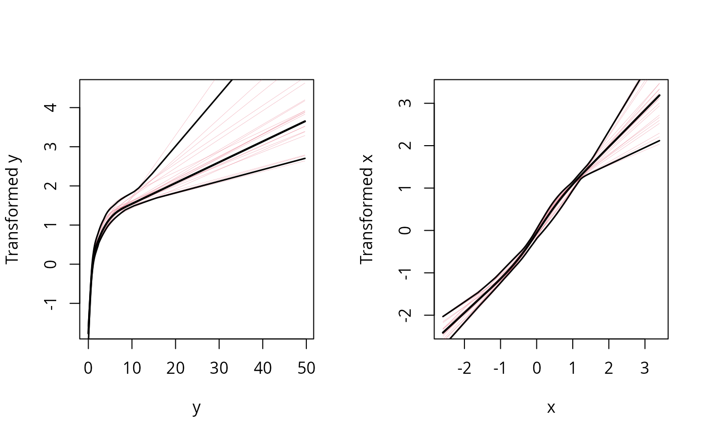
plot(f) # note log shape for y, linear for x. Good!
# Show fit of model by varying x1 on the x-axis and creating separate
# panels for x2 and x3. For x2 using only a few discrete values
newdat <- expand.grid(x1=seq(-2,2,length=100),x2=c(.25,.75),
x3=c('cat','dog','cow'))
yhat <- predict(f, newdat, statistic='fitted')
# statistic='mean' to get estimated mean rather than simple inverse trans.
xYplot(yhat ~ x1 | x2, groups=x3, type='l', data=newdat)
#> Error in eval(parse(text = yvname), data): object 'yhat' not found
if (FALSE) { # \dontrun{
# Another example, on hypothetical data
f <- areg.boot(response ~ I(age) + monotone(blood.pressure) + race)
# use I(response) to not transform the response variable
plot(f, conf.int=.9)
# Check distribution of residuals
plot(fitted(f), resid(f))
qqnorm(resid(f))
# Refit this model using ols so that we can draw a nomogram of it.
# The nomogram will show the linear predictor, median, mean.
# The last two are smearing estimators.
Function(f, type='individual') # create transformation functions
f.ols <- ols(.response(response) ~ age +
.blood.pressure(blood.pressure) + .race(race))
# Note: This model is almost exactly the same as f but there
# will be very small differences due to interpolation of
# transformations
meanr <- Mean(f) # create function of lp computing mean response
medr <- Quantile(f) # default quantile is .5
nomogram(f.ols, fun=list(Mean=meanr,Median=medr))
# Create S functions that will do the transformations
# This is a table look-up with linear interpolation
g <- Function(f)
plot(blood.pressure, g$blood.pressure(blood.pressure))
# produces the central curve in the last plot done by plot(f)
} # }
# Another simulated example, where y has a log-normal distribution
# with mean x and variance 1. Untransformed y thus has median
# exp(x) and mean exp(x + .5sigma^2) = exp(x + .5)
# First generate data from the model y = exp(x + epsilon),
# epsilon ~ Gaussian(0, 1)
set.seed(139)
n <- 1000
x <- rnorm(n)
y <- exp(x + rnorm(n))
f <- areg.boot(y ~ x, B=20)
#> 1
2
3
4
5
6
7
8
9
10
11
12
13
14
15
16
17
18
19
20
plot(f) # note log shape for y, linear for x. Good!
 xs <- c(-2, 0, 2)
d <- data.frame(x=xs)
predict(f, d, 'fitted')
#> Inverse Transformation
#> [1] 0.217 0.945 6.427
predict(f, d, 'median') # almost same; median residual=-.001
#> Median
#> [1] 0.216 0.944 6.412
exp(xs) # population medians
#> [1] 0.135 1.000 7.389
predict(f, d, 'mean')
#> Mean
#> [1] 0.261 1.675 10.113
exp(xs + .5) # population means
#> [1] 0.223 1.649 12.182
# Show how smearingEst works
res <- c(-1,0,1) # define residuals
y <- 1:5
ytrans <- log(y)
ys <- seq(.1,15,length=50)
trans.approx <- list(x=log(ys), y=ys)
options(digits=4)
smearingEst(ytrans, exp, res, 'fitted') # ignores res
#> Inverse Transformation
#> [1] 1 2 3 4 5
smearingEst(ytrans, trans.approx, res, 'fitted') # ignores res
#> Inverse Transformation
#> [1] 1.002 2.004 3.004 4.002 5.001
smearingEst(ytrans, exp, res, 'median') # median res=0
#> Median
#> [1] 1 2 3 4 5
smearingEst(ytrans, exp, res+.1, 'median') # median res=.1
#> Median
#> [1] 1.105 2.210 3.316 4.421 5.526
smearingEst(ytrans, trans.approx, res, 'median')
#> Median
#> [1] 1.002 2.004 3.004 4.002 5.001
smearingEst(ytrans, exp, res, 'mean')
#> Mean
#> [1] 1.362 2.724 4.086 5.448 6.810
mean(exp(ytrans[2] + res)) # should equal 2nd # above
#> [1] 2.724
smearingEst(ytrans, trans.approx, res, 'mean')
#> Mean
#> [1] 1.369 2.728 4.091 5.452 6.813
smearingEst(ytrans, trans.approx, res, mean)
#> mean
#> [1] 1.369 2.728 4.091 5.452 6.813
# Last argument can be any statistical function operating
# on a vector that returns a single value
xs <- c(-2, 0, 2)
d <- data.frame(x=xs)
predict(f, d, 'fitted')
#> Inverse Transformation
#> [1] 0.217 0.945 6.427
predict(f, d, 'median') # almost same; median residual=-.001
#> Median
#> [1] 0.216 0.944 6.412
exp(xs) # population medians
#> [1] 0.135 1.000 7.389
predict(f, d, 'mean')
#> Mean
#> [1] 0.261 1.675 10.113
exp(xs + .5) # population means
#> [1] 0.223 1.649 12.182
# Show how smearingEst works
res <- c(-1,0,1) # define residuals
y <- 1:5
ytrans <- log(y)
ys <- seq(.1,15,length=50)
trans.approx <- list(x=log(ys), y=ys)
options(digits=4)
smearingEst(ytrans, exp, res, 'fitted') # ignores res
#> Inverse Transformation
#> [1] 1 2 3 4 5
smearingEst(ytrans, trans.approx, res, 'fitted') # ignores res
#> Inverse Transformation
#> [1] 1.002 2.004 3.004 4.002 5.001
smearingEst(ytrans, exp, res, 'median') # median res=0
#> Median
#> [1] 1 2 3 4 5
smearingEst(ytrans, exp, res+.1, 'median') # median res=.1
#> Median
#> [1] 1.105 2.210 3.316 4.421 5.526
smearingEst(ytrans, trans.approx, res, 'median')
#> Median
#> [1] 1.002 2.004 3.004 4.002 5.001
smearingEst(ytrans, exp, res, 'mean')
#> Mean
#> [1] 1.362 2.724 4.086 5.448 6.810
mean(exp(ytrans[2] + res)) # should equal 2nd # above
#> [1] 2.724
smearingEst(ytrans, trans.approx, res, 'mean')
#> Mean
#> [1] 1.369 2.728 4.091 5.452 6.813
smearingEst(ytrans, trans.approx, res, mean)
#> mean
#> [1] 1.369 2.728 4.091 5.452 6.813
# Last argument can be any statistical function operating
# on a vector that returns a single value