Body Temperature Series of Beaver 1
beav1.RdReynolds (1994) describes a small part of a study of the long-term temperature dynamics of beaver Castor canadensis in north-central Wisconsin. Body temperature was measured by telemetry every 10 minutes for four females, but data from a one period of less than a day for each of two animals is used there.
beav1Format
The beav1 data frame has 114 rows and 4 columns.
This data frame contains the following columns:
dayDay of observation (in days since the beginning of 1990), December 12–13.
timeTime of observation, in the form
0330for 3.30am.tempMeasured body temperature in degrees Celsius.
activIndicator of activity outside the retreat.
Note
The observation at 22:20 is missing.
Source
P. S. Reynolds (1994) Time-series analyses of beaver body temperatures. Chapter 11 of Lange, N., Ryan, L., Billard, L., Brillinger, D., Conquest, L. and Greenhouse, J. eds (1994) Case Studies in Biometry. New York: John Wiley and Sons.
References
Venables, W. N. and Ripley, B. D. (2002) Modern Applied Statistics with S. Fourth edition. Springer.
See also
Examples
beav1 <- within(beav1,
hours <- 24*(day-346) + trunc(time/100) + (time%%100)/60)
plot(beav1$hours, beav1$temp, type="l", xlab="time",
ylab="temperature", main="Beaver 1")
usr <- par("usr"); usr[3:4] <- c(-0.2, 8); par(usr=usr)
lines(beav1$hours, beav1$activ, type="s", lty=2)
 temp <- ts(c(beav1$temp[1:82], NA, beav1$temp[83:114]),
start = 9.5, frequency = 6)
activ <- ts(c(beav1$activ[1:82], NA, beav1$activ[83:114]),
start = 9.5, frequency = 6)
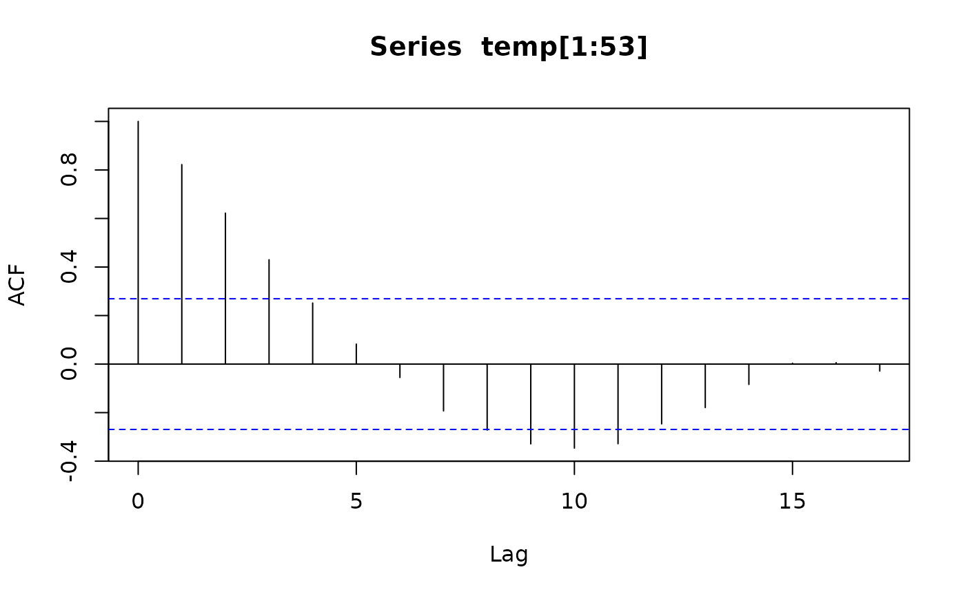
acf(temp[1:53])
temp <- ts(c(beav1$temp[1:82], NA, beav1$temp[83:114]),
start = 9.5, frequency = 6)
activ <- ts(c(beav1$activ[1:82], NA, beav1$activ[83:114]),
start = 9.5, frequency = 6)
acf(temp[1:53])
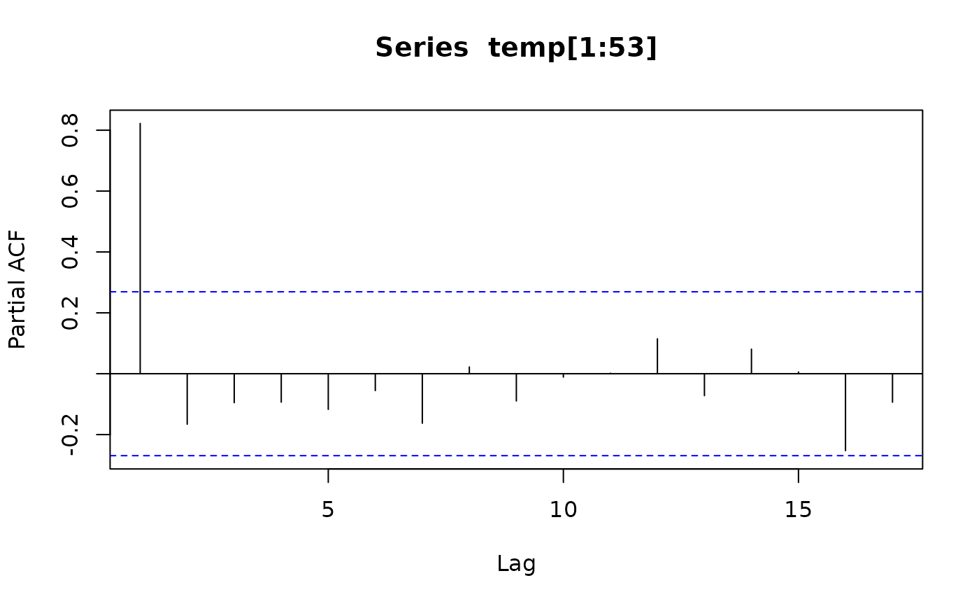
 acf(temp[1:53], type = "partial")
 ar(temp[1:53])
#>
#> Call:
#> ar(x = temp[1:53])
#>
#> Coefficients:
#> 1
#> 0.8222
#>
#> Order selected 1 sigma^2 estimated as 0.01011
act <- c(rep(0, 10), activ)
X <- cbind(1, act = act[11:125], act1 = act[10:124],
act2 = act[9:123], act3 = act[8:122])
alpha <- 0.80
stemp <- as.vector(temp - alpha*lag(temp, -1))
sX <- X[-1, ] - alpha * X[-115,]
beav1.ls <- lm(stemp ~ -1 + sX, na.action = na.omit)
summary(beav1.ls, correlation = FALSE)
#>
#> Call:
#> lm(formula = stemp ~ -1 + sX, na.action = na.omit)
#>
#> Residuals:
#> Min 1Q Median 3Q Max
#> -0.21317 -0.04317 0.00683 0.05483 0.37683
#>
#> Coefficients:
#> Estimate Std. Error t value Pr(>|t|)
#> sX 36.85587 0.03922 939.833 < 2e-16 ***
#> sXact 0.25400 0.03930 6.464 3.37e-09 ***
#> sXact1 0.17096 0.05100 3.352 0.00112 **
#> sXact2 0.16202 0.05147 3.148 0.00215 **
#> sXact3 0.10548 0.04310 2.448 0.01605 *
#> ---
#> Signif. codes: 0 ‘***’ 0.001 ‘**’ 0.01 ‘*’ 0.05 ‘.’ 0.1 ‘ ’ 1
#>
#> Residual standard error: 0.08096 on 104 degrees of freedom
#> (5 observations deleted due to missingness)
#> Multiple R-squared: 0.9999, Adjusted R-squared: 0.9999
#> F-statistic: 1.81e+05 on 5 and 104 DF, p-value: < 2.2e-16
#>
rm(temp, activ)
ar(temp[1:53])
#>
#> Call:
#> ar(x = temp[1:53])
#>
#> Coefficients:
#> 1
#> 0.8222
#>
#> Order selected 1 sigma^2 estimated as 0.01011
act <- c(rep(0, 10), activ)
X <- cbind(1, act = act[11:125], act1 = act[10:124],
act2 = act[9:123], act3 = act[8:122])
alpha <- 0.80
stemp <- as.vector(temp - alpha*lag(temp, -1))
sX <- X[-1, ] - alpha * X[-115,]
beav1.ls <- lm(stemp ~ -1 + sX, na.action = na.omit)
summary(beav1.ls, correlation = FALSE)
#>
#> Call:
#> lm(formula = stemp ~ -1 + sX, na.action = na.omit)
#>
#> Residuals:
#> Min 1Q Median 3Q Max
#> -0.21317 -0.04317 0.00683 0.05483 0.37683
#>
#> Coefficients:
#> Estimate Std. Error t value Pr(>|t|)
#> sX 36.85587 0.03922 939.833 < 2e-16 ***
#> sXact 0.25400 0.03930 6.464 3.37e-09 ***
#> sXact1 0.17096 0.05100 3.352 0.00112 **
#> sXact2 0.16202 0.05147 3.148 0.00215 **
#> sXact3 0.10548 0.04310 2.448 0.01605 *
#> ---
#> Signif. codes: 0 ‘***’ 0.001 ‘**’ 0.01 ‘*’ 0.05 ‘.’ 0.1 ‘ ’ 1
#>
#> Residual standard error: 0.08096 on 104 degrees of freedom
#> (5 observations deleted due to missingness)
#> Multiple R-squared: 0.9999, Adjusted R-squared: 0.9999
#> F-statistic: 1.81e+05 on 5 and 104 DF, p-value: < 2.2e-16
#>
rm(temp, activ)