Body Temperature Series of Beaver 2

Reynolds (1994) describes a small part of a study of the long-term temperature dynamics of beaver Castor canadensis in north-central Wisconsin. Body temperature was measured by telemetry every 10 minutes for four females, but data from a one period of less than a day for each of two animals is used there.

beav2

Format

The beav2 data frame has 100 rows and 4 columns. This data frame contains the following columns:

day

Day of observation (in days since the beginning of 1990), November 3–4.

time

Time of observation, in the form 0330 for 3.30am.

temp

Measured body temperature in degrees Celsius.

activ

Indicator of activity outside the retreat.

Source

P. S. Reynolds (1994) Time-series analyses of beaver body temperatures. Chapter 11 of Lange, N., Ryan, L., Billard, L., Brillinger, D., Conquest, L. and Greenhouse, J. eds (1994) Case Studies in Biometry. New York: John Wiley and Sons.

References

Venables, W. N. and Ripley, B. D. (2002) Modern Applied Statistics with S. Fourth edition. Springer.

See also

beav1

Examples

attach(beav2)
beav2$hours <- 24*(day-307) + trunc(time/100) + (time%%100)/60
plot(beav2$hours, beav2$temp, type = "l", xlab = "time",
   ylab = "temperature", main = "Beaver 2")
usr <- par("usr"); usr[3:4] <- c(-0.2, 8); par(usr = usr)
lines(beav2$hours, beav2$activ, type = "s", lty = 2)


temp <- ts(temp, start = 8+2/3, frequency = 6)
activ <- ts(activ, start = 8+2/3, frequency = 6)
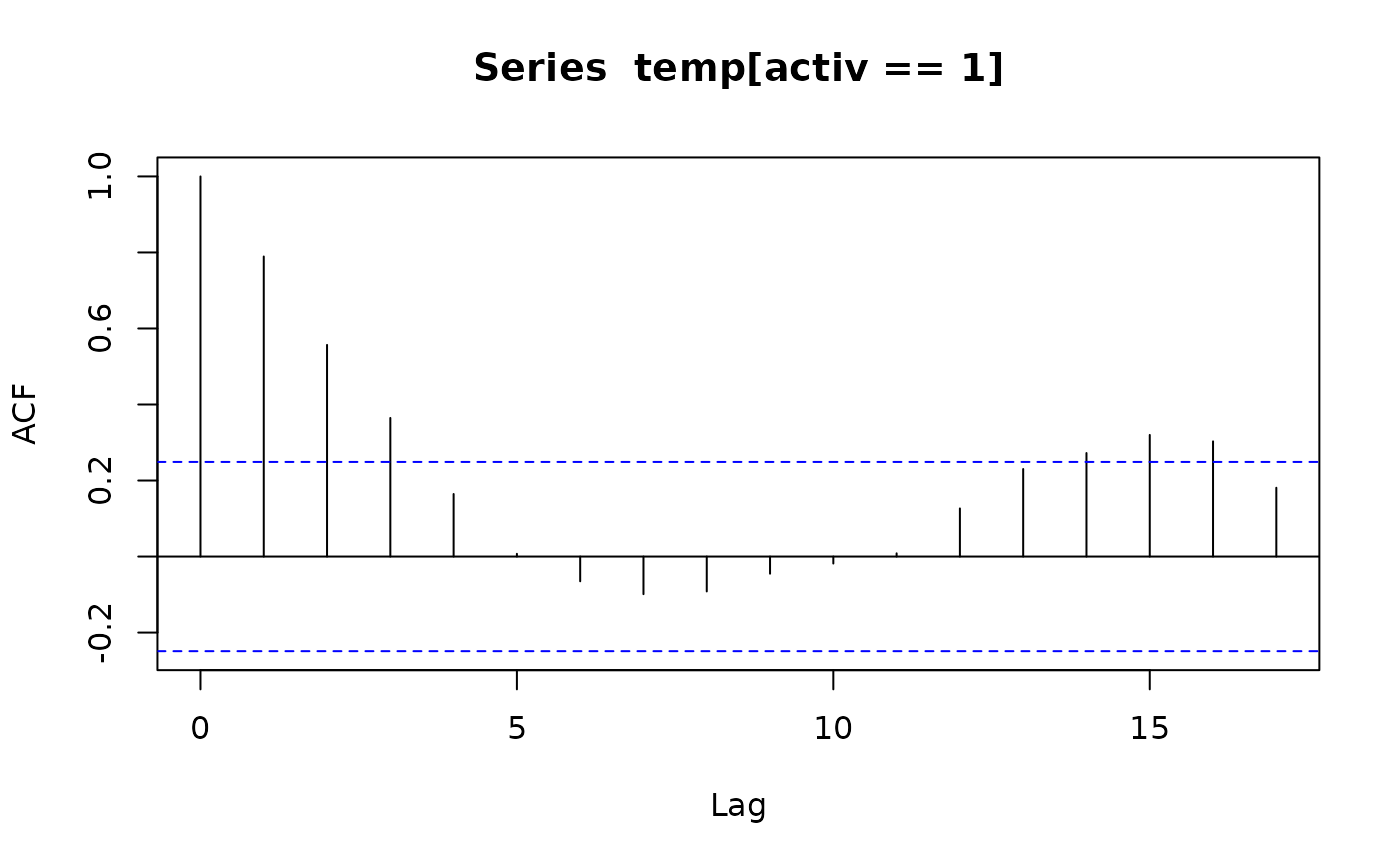
acf(temp[activ == 0]); acf(temp[activ == 1]) # also look at PACFs


ar(temp[activ == 0]); ar(temp[activ == 1])
#> 
#> Call:
#> ar(x = temp[activ == 0])
#> 
#> Coefficients:
#>      1  
#> 0.7392  
#> 
#> Order selected 1  sigma^2 estimated as  0.02011
#> 
#> Call:
#> ar(x = temp[activ == 1])
#> 
#> Coefficients:
#>      1  
#> 0.7894  
#> 
#> Order selected 1  sigma^2 estimated as  0.01792

arima(temp, order = c(1,0,0), xreg = activ)
#> 
#> Call:
#> arima(x = temp, order = c(1, 0, 0), xreg = activ)
#> 
#> Coefficients:
#>          ar1  intercept   activ
#>       0.8733    37.1920  0.6139
#> s.e.  0.0684     0.1187  0.1381
#> 
#> sigma^2 estimated as 0.01518:  log likelihood = 66.78,  aic = -125.55
dreg <- cbind(sin = sin(2*pi*beav2$hours/24), cos = cos(2*pi*beav2$hours/24))
arima(temp, order = c(1,0,0), xreg = cbind(active=activ, dreg))
#> 
#> Call:
#> arima(x = temp, order = c(1, 0, 0), xreg = cbind(active = activ, dreg))
#> 
#> Coefficients:
#>          ar1  intercept  active  dreg.sin  dreg.cos
#>       0.7905    37.1674  0.5322    -0.282    0.1201
#> s.e.  0.0681     0.0939  0.1282     0.105    0.0997
#> 
#> sigma^2 estimated as 0.01434:  log likelihood = 69.83,  aic = -127.67

## IGNORE_RDIFF_BEGIN
library(nlme) # for gls and corAR1
beav2.gls <- gls(temp ~ activ, data = beav2, correlation = corAR1(0.8),
                 method = "ML")
summary(beav2.gls)
#> Generalized least squares fit by maximum likelihood
#>   Model: temp ~ activ 
#>   Data: beav2 
#>         AIC       BIC   logLik
#>   -125.5505 -115.1298 66.77523
#> 
#> Correlation Structure: AR(1)
#>  Formula: ~1 
#>  Parameter estimate(s):
#>       Phi 
#> 0.8731771 
#> 
#> Coefficients:
#>                Value Std.Error  t-value p-value
#> (Intercept) 37.19195 0.1131328 328.7460       0
#> activ        0.61418 0.1087286   5.6487       0
#> 
#>  Correlation: 
#>       (Intr)
#> activ -0.582
#> 
#> Standardized residuals:
#>         Min          Q1         Med          Q3         Max 
#> -2.42080776 -0.61510520 -0.03573836  0.81641138  2.15153496 
#> 
#> Residual standard error: 0.2527856 
#> Degrees of freedom: 100 total; 98 residual
summary(update(beav2.gls, subset = 6:100))
#> Generalized least squares fit by maximum likelihood
#>   Model: temp ~ activ 
#>   Data: beav2 
#>   Subset: 6:100 
#>        AIC       BIC   logLik
#>   -124.981 -114.7654 66.49048
#> 
#> Correlation Structure: AR(1)
#>  Formula: ~1 
#>  Parameter estimate(s):
#>       Phi 
#> 0.8380448 
#> 
#> Coefficients:
#>                Value  Std.Error  t-value p-value
#> (Intercept) 37.25001 0.09634047 386.6496       0
#> activ        0.60277 0.09931904   6.0690       0
#> 
#>  Correlation: 
#>       (Intr)
#> activ -0.657
#> 
#> Standardized residuals:
#>        Min         Q1        Med         Q3        Max 
#> -2.0231494 -0.8910348 -0.1497564  0.7640939  2.2719468 
#> 
#> Residual standard error: 0.2188542 
#> Degrees of freedom: 95 total; 93 residual
detach("beav2"); rm(temp, activ)
## IGNORE_RDIFF_END