Tplyr Version 0.1.1
Welcome to Tplyr! This is the first full and stable release of our package. With this release comes a number of new enhancements, loads of new documentation, and our complete package qualification document.
If you’ve been keeping up, here are the things that we’ve added since the Beta release in July:
- Bug Fixes/Enhancements
- Count layers were re-factored to improve the execution efficiency
- Auto-precision now works without a
byvariable - Several new assertions have been added to give clearer error messages
- Treatment groups within the population data will produce columns in the resulting build, even if no records exist for that treatment group in the target dataset
- Risk difference variable names will now populate properly when a
colsargument is used - Data frame attributes are cleaned prior to processing to prevent any merge/bind warnings during processing
- Total values within count layers are properly filled when the resulting count is 0 (largely impacts risk-difference calculations)
- Feature additions
- Shift layers are here!
- Flexibility when filling missing values has been enhanced for descriptive statistic layers
- Layers can now be named, and those names can be used in
get_numeric_dataand the new functionget_statistics_datato get risk difference raw numbers. Data may also be filtered directly from both functions. - Default formats can now be set via options or at the table level, which allows you to eliminate a great deal of redundant code
As always, we welcome your feedback. If you spot a bug, would like to see a new feature, or if any documentation is unclear - submit an issue through GitHub right here.
What is Tplyr?
dplyr from tidyverse is a grammar of data manipulation. So what does that allow you to do? It gives you, as a data analyst, the capability to easily and intuitively approach the problem of manipulating your data into an analysis ready form. dplyr conceptually breaks things down into verbs that allow you to focus on what you want to do more than how you have to do it.
Tplyr is designed around a similar concept, but its focus is on building summary tables within the clinical world. In the pharmaceutical industry, a great deal of the data presented in the outputs we create are very similar. For the most part, most of these tables can be broken down into a few categories:
- Counting for event based variables or categories
- Shifting, which is just counting a change in state with a ‘from’ and a ‘to’
- Generating descriptive statistics around some continuous variable.
For many of the tables that go into a clinical submission, at least when considering safety outputs, the tables are made up of a combination of these approaches. Consider a demographics table - and let’s use an example from the PHUSE project Standard Analyses & Code Sharing - Analyses & Displays Associated with Demographics, Disposition, and Medications in Phase 2-4 Clinical Trials and Integrated Summary Documents.
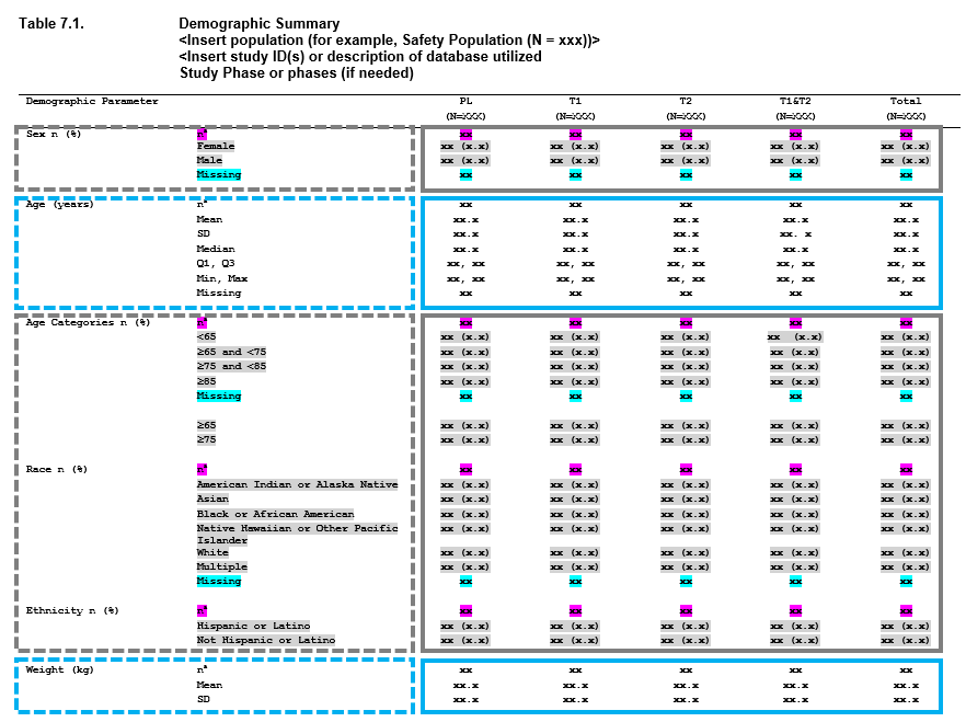
Demographics Table
When you look at this table, you can begin breaking this output down into smaller, redundant, components. These components can be viewed as ‘layers’, and the table as a whole is constructed by stacking the layers. The boxes in the image above represent how you can begin to conceptualize this.
- First we have Sex, which is made up of n (%) counts.
- Next we have Age as a continuous variable, where we have a number of descriptive statistics, including n, mean, standard deviation, median, quartile 1, quartile 3, min, max, and missing values.
- After that we have age, but broken into categories - so this is once again n (%) values.
- Race - more counting,
- Ethnicity - more counting
- Weight - and we’re back to descriptive statistics.
So we have one table, with 6 summaries (7 including the next page, not shown) - but only 2 different approaches to summaries being performed. In the same way that dplyr is a grammar of data manipulation, Tplyr aims to be a grammar of data summary. The goal of Tplyr is to allow you to program a summary table like you see it on the page, by breaking a larger problem into smaller ‘layers’, and combining them together like you see on the page.
Enough talking - let’s see some code. In these examples, we will be using data from the PHUSE Test Data Factory based on the original pilot project submission package. Note: You can see our replication of the CDISC pilot using the PHUSE Test Data Factory data here.
tplyr_table(adsl, TRT01P, where = SAFFL == "Y") %>%
  add_layer(
    group_desc(AGE, by = "Age (years)")
  ) %>%
  add_layer(
    group_count(AGEGR1, by = "Age Categories n (%)")
  ) %>%
  build()
#> # A tibble: 9 × 8
#>   row_label1           row_label2 var1_Placebo `var1_Xanomeli…` `var1_Xanomeli…`
#>   <chr>                <chr>      <chr>        <chr>            <chr>
#> 1 Age (years)          n          " 86"        " 84"            " 84"
#> 2 Age (years)          Mean (SD)  "75.2 ( 8.5… "74.4 ( 7.89)"   "75.7 ( 8.29)"
#> 3 Age (years)          Median     "76.0"       "76.0"           "77.5"
#> 4 Age (years)          Q1, Q3     "69.2, 81.8" "70.8, 80.0"     "71.0, 82.0"
#> 5 Age (years)          Min, Max   "52, 89"     "56, 88"         "51, 88"
#> 6 Age (years)          Missing    "  0"        "  0"            "  0"
#> 7 Age Categories n (%) <65        "14 ( 16.3%… "11 ( 13.1%)"    " 8 (  9.5%)"
#> 8 Age Categories n (%) >80        "30 ( 34.9%… "18 ( 21.4%)"    "29 ( 34.5%)"
#> 9 Age Categories n (%) 65-80      "42 ( 48.8%… "55 ( 65.5%)"    "47 ( 56.0%)"
#> # … with 3 more variables: ord_layer_index <int>, ord_layer_1 <int>,
#> #   ord_layer_2 <dbl>
The TL;DR
Here are some of the high level benefits of using Tplyr:
- Easy construction of table data using an intuitive syntax
- Smart string formatting for your numbers that’s easily specified by the user
- A great deal of flexibility in what is performed and how it’s presented, without specifying hundreds of parameters
- Extensibility (in the future…) - we’re going to open doors to allow you some level of customization.