Double Exponential Binomial Distribution Family Function
double.expbinomial.RdFits a double exponential binomial distribution by maximum likelihood estimation. The two parameters here are the mean and dispersion parameter.
double.expbinomial(lmean = "logitlink", ldispersion = "logitlink",
                   idispersion = 0.25, zero = "dispersion")
Arguments
- lmean, ldispersion
Link functions applied to the two parameters, called \(\mu\) and \(\theta\) respectively below. See
Linksfor more choices. The defaults cause the parameters to be restricted to \((0,1)\).- idispersion
Initial value for the dispersion parameter. If given, it must be in range, and is recyled to the necessary length. Use this argument if convergence failure occurs.
- zero
A vector specifying which linear/additive predictor is to be modelled as intercept-only. If assigned, the single value can be either
1or2. The default is to have a single dispersion parameter value. To model both parameters as functions of the covariates assignzero = NULL. SeeCommonVGAMffArgumentsfor more details.
Details
This distribution provides a way for handling overdispersion in a binary response. The double exponential binomial distribution belongs the family of double exponential distributions proposed by Efron (1986). Below, equation numbers refer to that original article. Briefly, the idea is that an ordinary one-parameter exponential family allows the addition of a second parameter \(\theta\) which varies the dispersion of the family without changing the mean. The extended family behaves like the original family with sample size changed from \(n\) to \(n\theta\). The extended family is an exponential family in \(\mu\) when \(n\) and \(\theta\) are fixed, and an exponential family in \(\theta\) when \(n\) and \(\mu\) are fixed. Having \(0 < \theta < 1\) corresponds to overdispersion with respect to the binomial distribution. See Efron (1986) for full details.
This VGAM family function implements an
approximation (2.10) to the exact density (2.4). It
replaces the normalizing constant by unity since the
true value nearly equals 1. The default model fitted is
\(\eta_1 = logit(\mu)\) and \(\eta_2
= logit(\theta)\). This restricts
both parameters to lie between 0 and 1, although the
dispersion parameter can be modelled over a larger parameter
space by assigning the arguments ldispersion and
edispersion.
Approximately, the mean (of \(Y\)) is \(\mu\). The effective sample size is the dispersion parameter multiplied by the original sample size, i.e., \(n\theta\). This family function uses Fisher scoring, and the two estimates are asymptotically independent because the expected information matrix is diagonal.
Value
An object of class "vglmff" (see
vglmff-class). The object is used by modelling
functions such as vglm.
References
Efron, B. (1986). Double exponential families and their use in generalized linear regression. Journal of the American Statistical Association, 81, 709–721.
Note
This function processes the input in the same way
as binomialff, however multiple responses are
not allowed (binomialff(multiple.responses = FALSE)).
Warning
Numerical difficulties can occur; if so, try using
idispersion.
See also
Examples
# This example mimics the example in Efron (1986).
# The results here differ slightly.
# Scale the variables
toxop <- transform(toxop,
phat = positive / ssize,
srainfall = scale(rainfall), # (6.1)
sN = scale(ssize)) # (6.2)
# A fit similar (should be identical) to Sec.6 of Efron (1986).
# But does not use poly(), and M = 1.25 here, as in (5.3)
cmlist <- list("(Intercept)" = diag(2),
"I(srainfall)" = rbind(1, 0),
"I(srainfall^2)" = rbind(1, 0),
"I(srainfall^3)" = rbind(1, 0),
"I(sN)" = rbind(0, 1),
"I(sN^2)" = rbind(0, 1))
fit <-
vglm(cbind(phat, 1 - phat) * ssize ~
I(srainfall) + I(srainfall^2) + I(srainfall^3) +
I(sN) + I(sN^2),
double.expbinomial(ldisp = "extlogitlink(min = 0, max = 1.25)",
idisp = 0.2, zero = NULL),
toxop, trace = TRUE, constraints = cmlist)
#> Iteration 1: loglikelihood = -473.41023
#> Iteration 2: loglikelihood = -472.665
#> Iteration 3: loglikelihood = -472.00972
#> Iteration 4: loglikelihood = -471.81556
#> Iteration 5: loglikelihood = -471.6183
#> Iteration 6: loglikelihood = -471.59167
#> Iteration 7: loglikelihood = -471.57862
#> Iteration 8: loglikelihood = -471.57585
#> Iteration 9: loglikelihood = -471.57487
#> Iteration 10: loglikelihood = -471.5746
#> Iteration 11: loglikelihood = -471.57452
#> Iteration 12: loglikelihood = -471.57449
#> Iteration 13: loglikelihood = -471.57449
# Now look at the results
coef(fit, matrix = TRUE)
#> logitlink(mu) extlogitlink(dispersion, min = 0, max = 1.25)
#> (Intercept) -0.0876428 0.6291300
#> I(srainfall) -0.6867008 0.0000000
#> I(srainfall^2) -0.1671289 0.0000000
#> I(srainfall^3) 0.2766119 0.0000000
#> I(sN) 0.0000000 0.4529937
#> I(sN^2) 0.0000000 -0.5863660
head(fitted(fit))
#> [,1]
#> [1,] 0.5406318
#> [2,] 0.4499732
#> [3,] 0.3884616
#> [4,] 0.4131199
#> [5,] 0.5483156
#> [6,] 0.5515432
summary(fit)
#>
#> Call:
#> vglm(formula = cbind(phat, 1 - phat) * ssize ~ I(srainfall) +
#> I(srainfall^2) + I(srainfall^3) + I(sN) + I(sN^2), family = double.expbinomial(ldisp = "extlogitlink(min = 0, max = 1.25)",
#> idisp = 0.2, zero = NULL), data = toxop, constraints = cmlist,
#> trace = TRUE)
#>
#> Coefficients:
#> Estimate Std. Error z value Pr(>|z|)
#> (Intercept):1 -0.08764 0.14177 -0.618 0.53643
#> (Intercept):2 0.62913 0.87260 0.721 0.47092
#> I(srainfall) -0.68670 0.23225 -2.957 0.00311 **
#> I(srainfall^2) -0.16713 0.10930 -1.529 0.12624
#> I(srainfall^3) 0.27661 0.08644 3.200 0.00137 **
#> I(sN) 0.45299 1.03977 0.436 0.66308
#> I(sN^2) -0.58637 0.53422 -1.098 0.27238
#> ---
#> Signif. codes: 0 ‘***’ 0.001 ‘**’ 0.01 ‘*’ 0.05 ‘.’ 0.1 ‘ ’ 1
#>
#> Names of linear predictors: logitlink(mu),
#> extlogitlink(dispersion, min = 0, max = 1.25)
#>
#> Log-likelihood: -471.5745 on 61 degrees of freedom
#>
#> Number of Fisher scoring iterations: 13
#>
#> No Hauck-Donner effect found in any of the estimates
#>
vcov(fit)
#> (Intercept):1 (Intercept):2 I(srainfall) I(srainfall^2)
#> (Intercept):1 2.009784e-02 -1.316227e-19 1.575495e-03 -9.186354e-03
#> (Intercept):2 -1.316227e-19 7.614306e-01 1.595870e-18 5.385259e-19
#> I(srainfall) 1.575495e-03 1.595870e-18 5.394044e-02 8.584228e-03
#> I(srainfall^2) -9.186354e-03 5.385259e-19 8.584228e-03 1.194605e-02
#> I(srainfall^3) 1.440713e-03 -6.826596e-19 -1.746804e-02 -5.894585e-03
#> I(sN) -7.972138e-20 6.334727e-01 9.665884e-19 3.261749e-19
#> I(sN^2) 7.791228e-20 -3.763901e-01 -9.446539e-19 -3.187731e-19
#> I(srainfall^3) I(sN) I(sN^2)
#> (Intercept):1 1.440713e-03 -7.972138e-20 7.791228e-20
#> (Intercept):2 -6.826596e-19 6.334727e-01 -3.763901e-01
#> I(srainfall) -1.746804e-02 9.665884e-19 -9.446539e-19
#> I(srainfall^2) -5.894585e-03 3.261749e-19 -3.187731e-19
#> I(srainfall^3) 7.472242e-03 -4.134740e-19 4.040911e-19
#> I(sN) -4.134740e-19 1.081116e+00 -5.229643e-01
#> I(sN^2) 4.040911e-19 -5.229643e-01 2.853935e-01
sqrt(diag(vcov(fit))) # Standard errors
#> (Intercept):1 (Intercept):2 I(srainfall) I(srainfall^2) I(srainfall^3)
#> 0.14176683 0.87259991 0.23225082 0.10929800 0.08644213
#> I(sN) I(sN^2)
#> 1.03976738 0.53422232
# Effective sample size (not quite the last column of Table 1)
head(predict(fit))
#> logitlink(mu) extlogitlink(dispersion, min = 0, max = 1.25)
#> 1 0.1628865 -0.008940524
#> 2 -0.2007791 0.294623793
#> 3 -0.4537834 0.047331202
#> 4 -0.3510827 0.294623793
#> 5 0.1938674 -0.128297183
#> 6 0.2069076 0.047331202
Dispersion <- extlogitlink(predict(fit)[,2], min = 0, max = 1.25,
inverse = TRUE)
c(round(weights(fit, type = "prior") * Dispersion, digits = 1))
#> [1] 2.5 7.2 3.2 7.2 1.2 3.2 5.5 15.3 3.9 7.2 19.9 0.6 25.2 18.1 0.6
#> [16] 8.0 0.6 34.1 6.3 14.4 8.9 0.6 8.0 12.9 34.7 12.5 8.2 9.8 33.5 15.0
#> [31] 9.8 7.2 3.9 30.4
# Ordinary logistic regression (gives same results as (6.5))
ofit <- vglm(cbind(phat, 1 - phat) * ssize ~
I(srainfall) + I(srainfall^2) + I(srainfall^3),
binomialff, toxop, trace = TRUE)
#> Iteration 1: deviance = 62.708824
#> Iteration 2: deviance = 62.634603
#> Iteration 3: deviance = 62.634602
# Same as fit but it uses poly(), and can be plotted (cf. Fig.1)
cmlist2 <- list("(Intercept)" = diag(2),
"poly(srainfall, degree = 3)" = rbind(1, 0),
"poly(sN, degree = 2)" = rbind(0, 1))
fit2 <-
vglm(cbind(phat, 1 - phat) * ssize ~
poly(srainfall, degree = 3) + poly(sN, degree = 2),
double.expbinomial(ldisp = "extlogitlink(min = 0, max = 1.25)",
idisp = 0.2, zero = NULL),
toxop, trace = TRUE, constraints = cmlist2)
#> Iteration 1: loglikelihood = -473.41023
#> Iteration 2: loglikelihood = -472.665
#> Iteration 3: loglikelihood = -472.00972
#> Iteration 4: loglikelihood = -471.81556
#> Iteration 5: loglikelihood = -471.6183
#> Iteration 6: loglikelihood = -471.59167
#> Iteration 7: loglikelihood = -471.57862
#> Iteration 8: loglikelihood = -471.57585
#> Iteration 9: loglikelihood = -471.57487
#> Iteration 10: loglikelihood = -471.5746
#> Iteration 11: loglikelihood = -471.57452
#> Iteration 12: loglikelihood = -471.57449
#> Iteration 13: loglikelihood = -471.57449
if (FALSE) par(mfrow = c(1, 2)) # Cf. Fig.1
plot(as(fit2, "vgam"), se = TRUE, lcol = "blue", scol = "orange")
#> Error in eval(predvars, data, env): object 'srainfall' not found
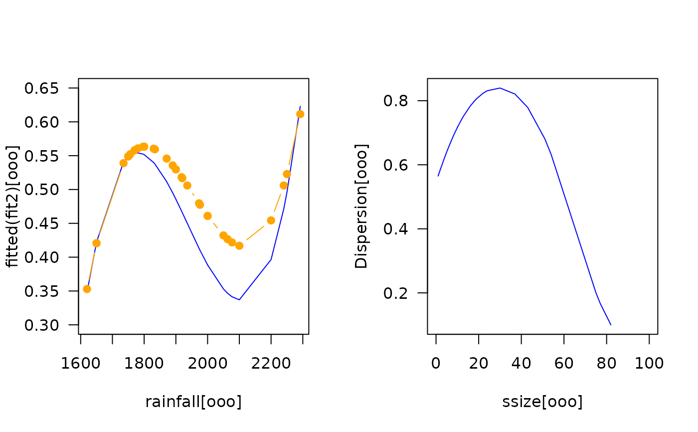
# Cf. Figure 1(a)
par(mfrow = c(1,2))
ooo <- with(toxop, sort.list(rainfall))
with(toxop, plot(rainfall[ooo], fitted(fit2)[ooo], type = "l",
col = "blue", las = 1, ylim = c(0.3, 0.65)))
with(toxop, points(rainfall[ooo], fitted(ofit)[ooo],
col = "orange", type = "b", pch = 19))
# Cf. Figure 1(b)
ooo <- with(toxop, sort.list(ssize))
with(toxop, plot(ssize[ooo], Dispersion[ooo], type = "l",
col = "blue", las = 1, xlim = c(0, 100))) # \dontrun{}