Logit Link Function

Computes the logit transformation, including its inverse and the first nine derivatives.

logitlink(theta, bvalue = NULL, inverse = FALSE, deriv = 0,
    short = TRUE, tag = FALSE)
extlogitlink(theta, min = 0, max = 1, bminvalue = NULL,
    bmaxvalue = NULL, inverse = FALSE, deriv = 0,
    short = TRUE, tag = FALSE)

Arguments

theta

Numeric or character. See below for further details.

bvalue, bminvalue, bmaxvalue

See Links. These are boundary values. For extlogitlink, values of theta less than or equal to \(A\) or greater than or equal to \(B\) can be replaced by bminvalue and bmaxvalue.

min, max

For extlogitlink, min gives \(A\), max gives \(B\), and for out of range values, bminvalue and bmaxvalue.

inverse, deriv, short, tag

Details at Links.

Details

The logit link function is very commonly used for parameters that lie in the unit interval. It is the inverse CDF of the logistic distribution. Numerical values of theta close to 0 or 1 or out of range result in Inf, -Inf, NA or NaN.

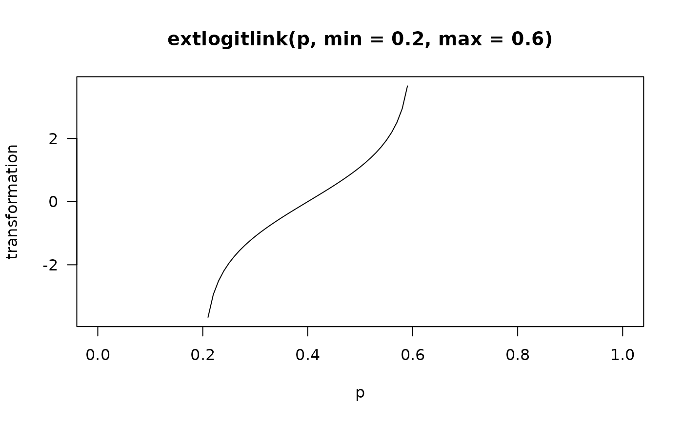
The extended logit link function extlogitlink should be used more generally for parameters that lie in the interval \((A,B)\), say. The formula is $$\log((\theta-A)/(B-\theta))$$ and the default values for \(A\) and \(B\) correspond to the ordinary logit function. Numerical values of theta close to \(A\) or \(B\) or out of range result in Inf, -Inf, NA or NaN. However these can be replaced by values \(bminvalue\) and \(bmaxvalue\) first before computing the link function.

Value

For logitlink with deriv = 0, the logit of theta, i.e., log(theta/(1-theta)) when inverse = FALSE, and if inverse = TRUE then exp(theta)/(1+exp(theta)).

For deriv = 1, then the function returns d eta / d theta as a function of theta if inverse = FALSE, else if inverse = TRUE then it returns the reciprocal.

Here, all logarithms are natural logarithms, i.e., to base e.

References

McCullagh, P. and Nelder, J. A. (1989). Generalized Linear Models, 2nd ed. London: Chapman & Hall.

Author

Thomas W. Yee

Note

Numerical instability may occur when theta is close to 1 or 0 (for logitlink), or close to \(A\) or \(B\) for extlogitlink. One way of overcoming this is to use, e.g., bvalue.

In terms of the threshold approach with cumulative probabilities for an ordinal response this link function corresponds to the univariate logistic distribution (see logistic).

See also

Links, alogitlink, asinlink, logitoffsetlink, probitlink, clogloglink, cauchitlink, logistic1, loglink, Logistic, multilogitlink.

Examples

p <- seq(0.01, 0.99, by = 0.01)
logitlink(p)
#>  [1] -4.59511985 -3.89182030 -3.47609869 -3.17805383 -2.94443898 -2.75153531
#>  [7] -2.58668934 -2.44234704 -2.31363493 -2.19722458 -2.09074110 -1.99243016
#> [13] -1.90095876 -1.81528997 -1.73460106 -1.65822808 -1.58562726 -1.51634749
#> [19] -1.45001018 -1.38629436 -1.32492541 -1.26566637 -1.20831121 -1.15267951
#> [25] -1.09861229 -1.04596856 -0.99462258 -0.94446161 -0.89538405 -0.84729786
#> [31] -0.80011930 -0.75377180 -0.70818506 -0.66329422 -0.61903921 -0.57536414
#> [37] -0.53221681 -0.48954823 -0.44731222 -0.40546511 -0.36396538 -0.32277339
#> [43] -0.28185115 -0.24116206 -0.20067070 -0.16034265 -0.12014431 -0.08004271
#> [49] -0.04000533  0.00000000  0.04000533  0.08004271  0.12014431  0.16034265
#> [55]  0.20067070  0.24116206  0.28185115  0.32277339  0.36396538  0.40546511
#> [61]  0.44731222  0.48954823  0.53221681  0.57536414  0.61903921  0.66329422
#> [67]  0.70818506  0.75377180  0.80011930  0.84729786  0.89538405  0.94446161
#> [73]  0.99462258  1.04596856  1.09861229  1.15267951  1.20831121  1.26566637
#> [79]  1.32492541  1.38629436  1.45001018  1.51634749  1.58562726  1.65822808
#> [85]  1.73460106  1.81528997  1.90095876  1.99243016  2.09074110  2.19722458
#> [91]  2.31363493  2.44234704  2.58668934  2.75153531  2.94443898  3.17805383
#> [97]  3.47609869  3.89182030  4.59511985
max(abs(logitlink(logitlink(p), inverse = TRUE) - p))  # 0?
#> [1] 1.110223e-16

p <- c(seq(-0.02, 0.02, by = 0.01), seq(0.97, 1.02, by = 0.01))
logitlink(p)  # Has NAs
#>  [1]       NaN       NaN      -Inf -4.595120 -3.891820  3.476099  3.891820
#>  [8]  4.595120       Inf       NaN       NaN
logitlink(p, bvalue = .Machine$double.eps)  # Has no NAs
#>  [1] -36.043653 -36.043653 -36.043653  -4.595120  -3.891820   3.476099
#>  [7]   3.891820   4.595120  36.043653  36.043653  36.043653

p <- seq(0.9, 2.2, by = 0.1)
extlogitlink(p, min = 1, max = 2,
             bminvalue = 1 + .Machine$double.eps,
             bmaxvalue = 2 - .Machine$double.eps)  # Has no NAs
#>  [1] -36.0436534 -36.0436534  -2.1972246  -1.3862944  -0.8472979  -0.4054651
#>  [7]   0.0000000   0.4054651   0.8472979   1.3862944   2.1972246  36.0436534
#> [13]  36.0436534  36.0436534

if (FALSE)  par(mfrow = c(2,2), lwd = (mylwd <- 2))
y <- seq(-4, 4, length = 100)
p <- seq(0.01, 0.99, by = 0.01)
for (d in 0:1) {
  myinv <- (d > 0)
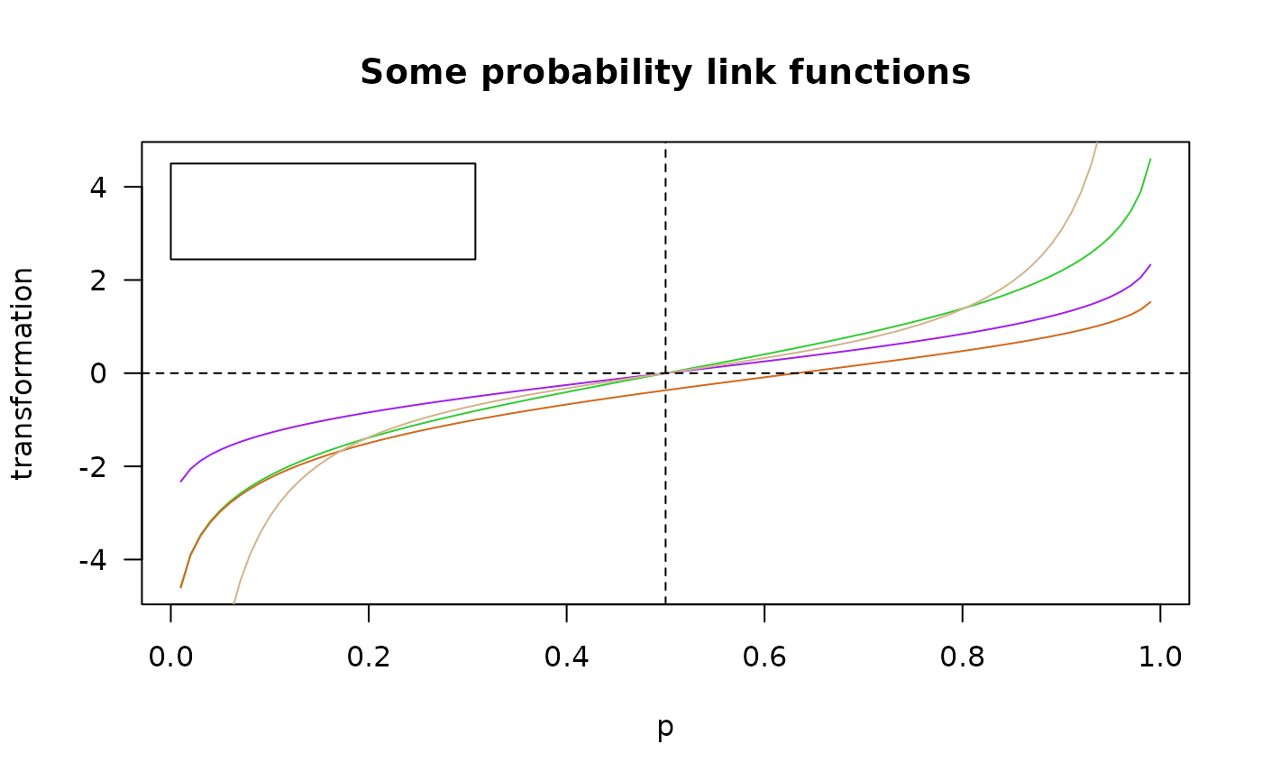
  matplot(p, cbind( logitlink(p, deriv = d, inv = myinv),
                   probitlink(p, deriv = d, inv = myinv)), las = 1,
          type = "n", col = "purple", ylab = "transformation",
          main = if (d ==  0) "Some probability link functions"
          else "1 / first derivative")
  lines(p,   logitlink(p, deriv = d, inverse = myinv), col = "limegreen")
  lines(p,  probitlink(p, deriv = d, inverse = myinv), col = "purple")
  lines(p, clogloglink(p, deriv = d, inverse = myinv), col = "chocolate")
  lines(p, cauchitlink(p, deriv = d, inverse = myinv), col = "tan")
  if (d ==  0) {
    abline(v = 0.5, h = 0, lty = "dashed")
    legend(0, 4.5, c("logitlink", "probitlink",
           "clogloglink", "cauchitlink"), col = c("limegreen", "purple",
           "chocolate", "tan"), lwd = mylwd)
  } else
    abline(v = 0.5, lty = "dashed")
}

#> Error: object 'mylwd' not found

for (d in 0) {
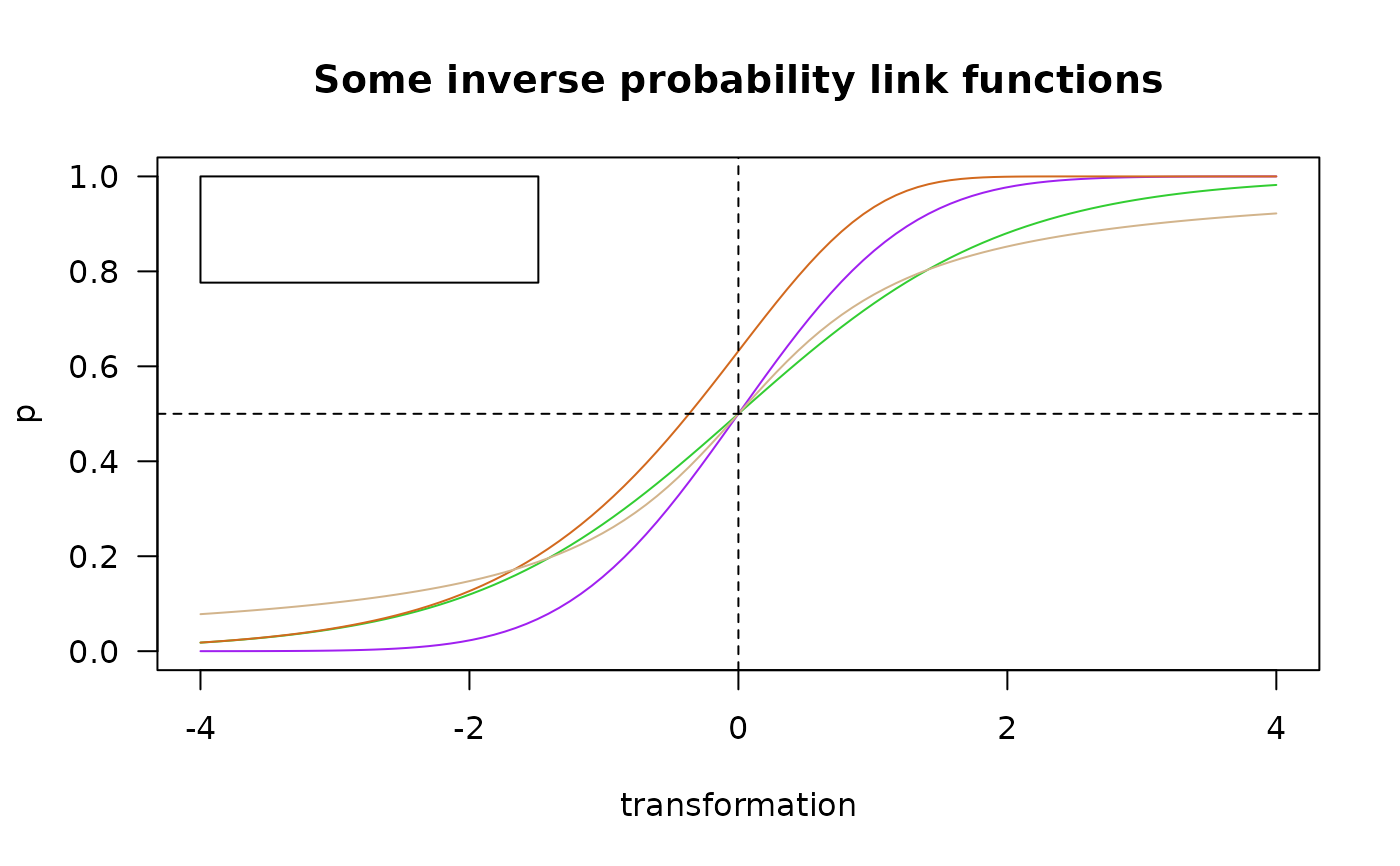
  matplot(y, cbind(logitlink(y, deriv = d, inverse = TRUE),
                   probitlink(y, deriv = d, inverse = TRUE)), las = 1,
          type = "n", col = "purple", xlab = "transformation", ylab = "p",
          main = if (d ==  0) "Some inverse probability link functions"
          else "First derivative")
  lines(y,   logitlink(y, deriv = d, inv = TRUE), col = "limegreen")
  lines(y,  probitlink(y, deriv = d, inv = TRUE), col = "purple")
  lines(y, clogloglink(y, deriv = d, inv = TRUE), col = "chocolate")
  lines(y, cauchitlink(y, deriv = d, inv = TRUE), col = "tan")
  if (d ==  0) {
    abline(h = 0.5, v = 0, lty = "dashed")
    legend(-4, 1, c("logitlink", "probitlink", "clogloglink",
           "cauchitlink"), col = c("limegreen", "purple",
           "chocolate", "tan"), lwd = mylwd)
  }
}

#> Error: object 'mylwd' not found

p <- seq(0.21, 0.59, by = 0.01)
plot(p, extlogitlink(p, min = 0.2, max = 0.6), xlim = c(0, 1),
     type = "l", col = "black", ylab = "transformation",
     las = 1, main = "extlogitlink(p, min = 0.2, max = 0.6)")

par(lwd = 1)
 # \dontrun{}