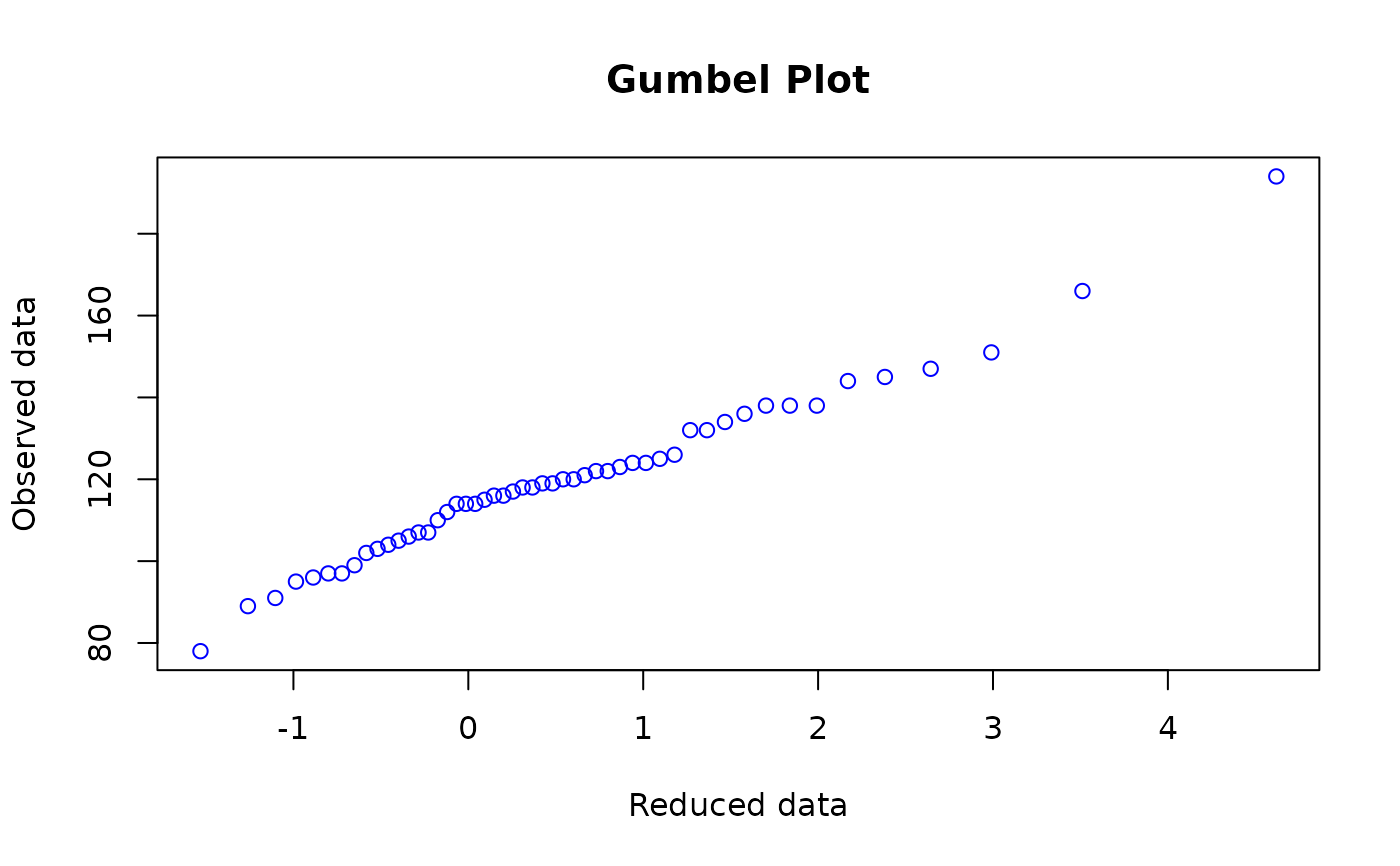
Gumbel Plot

Produces a Gumbel plot, a diagnostic plot for checking whether the data appears to be from a Gumbel distribution.

guplot(object, ...)
guplot.default(y, main = "Gumbel Plot",
    xlab = "Reduced data", ylab = "Observed data", type = "p", ...)
guplot.vlm(object, ...)

Arguments

y

A numerical vector. NAs etc. are not allowed.

main

Character. Overall title for the plot.

xlab

Character. Title for the x axis.

ylab

Character. Title for the y axis.

type

Type of plot. The default means points are plotted.

object

An object that inherits class "vlm", usually of class vglm-class or vgam-class.

...

Graphical argument passed into plot. See par for an exhaustive list. The arguments xlim and ylim are particularly useful.

Details

If $Y$ has a Gumbel distribution then plotting the sorted values $y_i$ versus the reduced values $r_i$ should appear linear. The reduced values are given by $$r_i = -\log(-\log(p_i)) $$ where $p_i$ is the $i$th plotting position, taken here to be $(i-0.5)/n$. Here, $n$ is the number of observations. Curvature upwards/downwards may indicate a Frechet/Weibull distribution, respectively. Outliers may also be detected using this plot.

The function guplot is generic, and guplot.default and guplot.vlm are some methods functions for Gumbel plots.

Value

A list is returned invisibly with the following components.

x: The reduced data.
y: The sorted y data.

References

Coles, S. (2001). An Introduction to Statistical Modeling of Extreme Values. London: Springer-Verlag.

Gumbel, E. J. (1958). Statistics of Extremes. New York, USA: Columbia University Press.

Author

T. W. Yee

Note

The Gumbel distribution is a special case of the GEV distribution with shape parameter equal to zero.

Examples

if (FALSE) guplot(rnorm(500), las = 1) -> ii
names(ii)
#> Error: object 'ii' not found

guplot(with(venice, r1), col = "blue")  # Venice sea levels data

 # \dontrun{}