Gumbel Regression Family Function
gumbel.RdMaximum likelihood estimation of the 2-parameter Gumbel distribution.
Arguments
- llocation, lscale
Parameter link functions for \(\mu\) and \(\sigma\). See
Linksfor more choices.- iscale
Numeric and positive. Optional initial value for \(\sigma\). Recycled to the appropriate length. In general, a larger value is better than a smaller value. A
NULLmeans an initial value is computed internally.- R
Numeric. Maximum number of values possible. See Details for more details.
- percentiles
Numeric vector of percentiles used for the fitted values. Values should be between 0 and 100. This argument uses the argument
Rif assigned. Ifpercentiles = NULLthen the mean will be returned as the fitted values.- mpv
Logical. If
mpv = TRUEthen the median predicted value (MPV) is computed and returned as the (last) column of the fitted values. This argument is ignored ifpercentiles = NULL. See Details for more details.
- zero
A vector specifying which linear/additive predictors are modelled as intercepts only. The value (possibly values) can be from the set {1, 2} corresponding respectively to \(\mu\) and \(\sigma\). By default all linear/additive predictors are modelled as a linear combination of the explanatory variables. See
CommonVGAMffArgumentsfor more details.
Details
The Gumbel distribution is a generalized extreme value (GEV)
distribution with shape parameter \(\xi = 0\).
Consequently it is more easily estimated than the GEV.
See gev for more details.
The quantity \(R\) is the maximum number of observations possible,
for example, in the Venice data below, the top 10 daily values
are recorded for each year, therefore \(R = 365\) because there are
about 365 days per year.
The MPV is the value of the response such that the probability
of obtaining a value greater than the MPV is 0.5 out of
\(R\) observations.
For the Venice data, the MPV is the sea level such that there
is an even chance that the highest level for a particular year
exceeds the MPV.
If mpv = TRUE then the column labelled "MPV" contains
the MPVs when fitted() is applied to the fitted object.
The formula for the mean of a response \(Y\) is
\(\mu+\sigma \times Euler\) where \(Euler\) is a constant
that has value approximately equal to 0.5772.
The formula for the percentiles are (if R is not given)
\(\mu-\sigma \times \log[-\log(P/100)]\)
where \(P\) is the percentile argument value(s).
If R is given then the percentiles are
\(\mu-\sigma \times \log[R(1-P/100)]\).
Value
An object of class "vglmff" (see vglmff-class).
The object is used by modelling functions such as vglm,
and vgam.
References
Yee, T. W. and Stephenson, A. G. (2007). Vector generalized linear and additive extreme value models. Extremes, 10, 1–19.
Smith, R. L. (1986). Extreme value theory based on the r largest annual events. Journal of Hydrology, 86, 27–43.
Rosen, O. and Cohen, A. (1996). Extreme percentile regression. In: Haerdle, W. and Schimek, M. G. (eds.), Statistical Theory and Computational Aspects of Smoothing: Proceedings of the COMPSTAT '94 Satellite Meeting held in Semmering, Austria, 27–28 August 1994, pp.200–214, Heidelberg: Physica-Verlag.
Coles, S. (2001). An Introduction to Statistical Modeling of Extreme Values. London: Springer-Verlag.
Warning
When R is not given (the default) the fitted percentiles are
that of the data, and not of the
overall population. For example, in the example below, the 50
percentile is approximately the running median through the data,
however, the data are the highest sea level measurements recorded each
year (it therefore equates to the median predicted value or MPV).
Note
Like many other usual VGAM family functions,
gumbelff() handles (independent) multiple responses.
gumbel() can handle
more of a
multivariate response, i.e., a
matrix with more than one column. Each row of the matrix is
sorted into descending order.
Missing values in the response are allowed but require
na.action = na.pass. The response matrix needs to be
padded with any missing values. With a multivariate response
one has a matrix y, say, where
y[, 2] contains the second order statistics, etc.
Examples
# Example 1: Simulated data
gdata <- data.frame(y1 = rgumbel(n = 1000, loc = 100, scale = exp(1)))
fit1 <- vglm(y1 ~ 1, gumbelff(perc = NULL), data = gdata, trace = TRUE)
#> Iteration 1: loglikelihood = -2597.9601
#> Iteration 2: loglikelihood = -2587.7893
#> Iteration 3: loglikelihood = -2587.6911
#> Iteration 4: loglikelihood = -2587.6911
coef(fit1, matrix = TRUE)
#> location loglink(scale)
#> (Intercept) 100.0273 1.012899
Coef(fit1)
#> location scale
#> 100.027323 2.753572
head(fitted(fit1))
#> [,1]
#> [1,] 101.6167
#> [2,] 101.6167
#> [3,] 101.6167
#> [4,] 101.6167
#> [5,] 101.6167
#> [6,] 101.6167
with(gdata, mean(y1))
#> [1] 101.6101
# Example 2: Venice data
(fit2 <- vglm(cbind(r1, r2, r3, r4, r5) ~ year, data = venice,
gumbel(R = 365, mpv = TRUE), trace = TRUE))
#> Iteration 1: loglikelihood = -719.30727
#> Iteration 2: loglikelihood = -706.68238
#> Iteration 3: loglikelihood = -705.03014
#> Iteration 4: loglikelihood = -705.02544
#> Iteration 5: loglikelihood = -705.02542
#> Iteration 6: loglikelihood = -705.02542
#>
#> Call:
#> vglm(formula = cbind(r1, r2, r3, r4, r5) ~ year, family = gumbel(R = 365,
#> mpv = TRUE), data = venice, trace = TRUE)
#>
#>
#> Coefficients:
#> (Intercept):1 (Intercept):2 year:1 year:2
#> -8.447828e+02 -1.495767e-01 4.912844e-01 1.378431e-03
#>
#> Degrees of Freedom: 102 Total; 98 Residual
#> Log-likelihood: -705.0254
head(fitted(fit2))
#> 95% 99% MPV
#> 1 68.07416 87.92128 108.4072
#> 2 68.51604 88.39054 108.9047
#> 3 68.95786 88.85977 109.4022
#> 4 69.39961 89.32897 109.8998
#> 5 69.84129 89.79814 110.3973
#> 6 70.28290 90.26728 110.8949
coef(fit2, matrix = TRUE)
#> location loglink(scale)
#> (Intercept) -844.7827502 -0.149576688
#> year 0.4912844 0.001378431
sqrt(diag(vcov(summary(fit2)))) # Standard errors
#> (Intercept):1 (Intercept):2 year:1 year:2
#> 1.975734e+02 7.653386e+00 1.010370e-01 3.912663e-03
# Example 3: Try a nonparametric fit ---------------------
# Use the entire data set, including missing values
# Same as as.matrix(venice[, paste0("r", 1:10)]):
Y <- Select(venice, "r", sort = FALSE)
fit3 <- vgam(Y ~ s(year, df = 3), gumbel(R = 365, mpv = TRUE),
data = venice, trace = TRUE, na.action = na.pass)
#> VGAM s.vam loop 1 : loglikelihood = -1137.5884
#> VGAM s.vam loop 2 : loglikelihood = -1088.6181
#> VGAM s.vam loop 3 : loglikelihood = -1079.7142
#> VGAM s.vam loop 4 : loglikelihood = -1078.882
#> VGAM s.vam loop 5 : loglikelihood = -1078.7252
#> VGAM s.vam loop 6 : loglikelihood = -1078.713
#> VGAM s.vam loop 7 : loglikelihood = -1078.7071
#> VGAM s.vam loop 8 : loglikelihood = -1078.707
#> VGAM s.vam loop 9 : loglikelihood = -1078.7066
#> VGAM s.vam loop 10 : loglikelihood = -1078.7066
depvar(fit3)[4:5, ] # NAs used to pad the matrix
#> r1 r2 r3 r4 r5 r6 r7 r8 r9 r10
#> 4 116 113 91 91 91 89 88 88 86 81
#> 5 115 107 105 101 93 91 NA NA NA NA
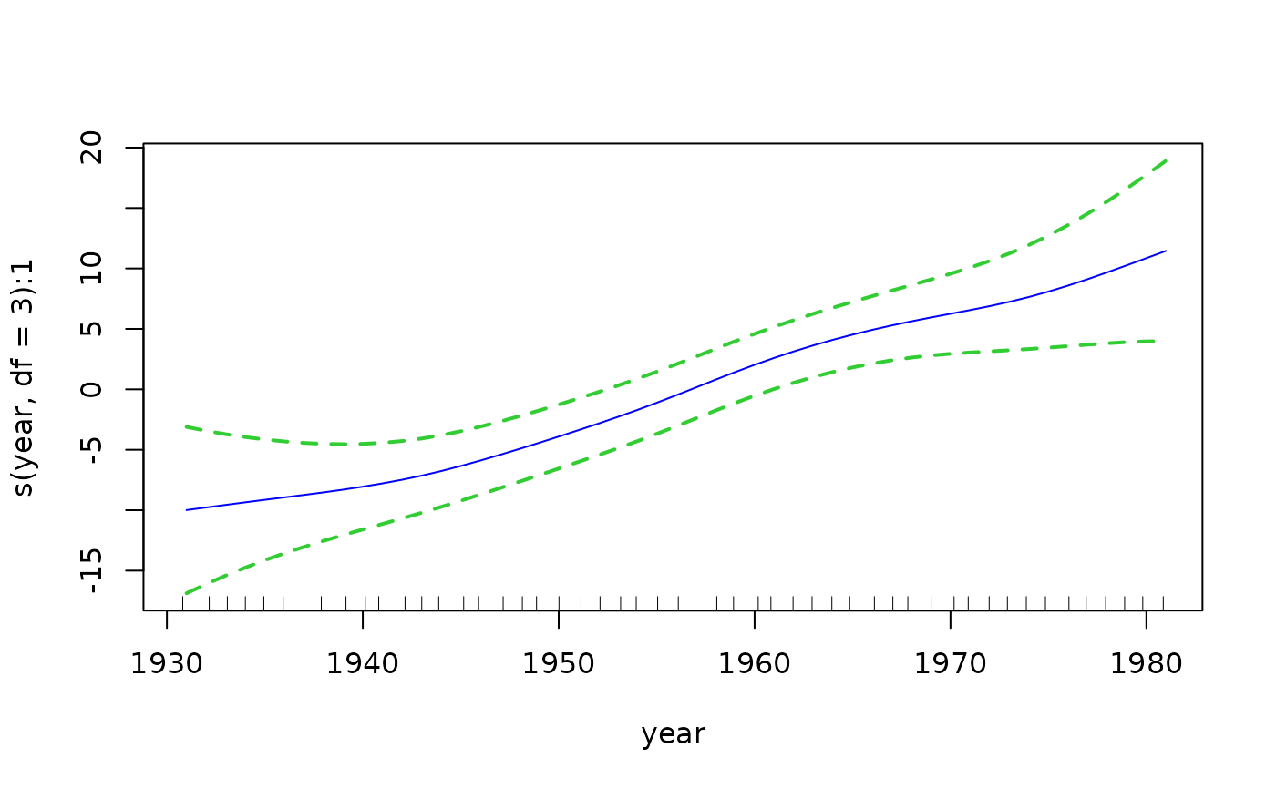
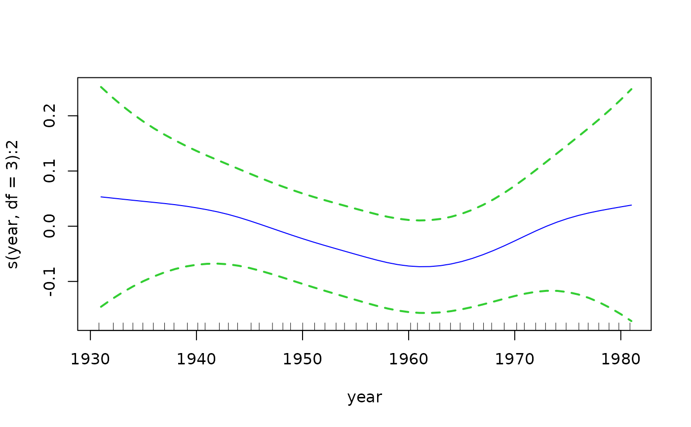
if (FALSE) # Plot the component functions
par(mfrow = c(2, 3), mar = c(6, 4, 1, 2) + 0.3, xpd = TRUE)
plot(fit3, se = TRUE, lcol = "blue", scol = "limegreen", lty = 1,
lwd = 2, slwd = 2, slty = "dashed")
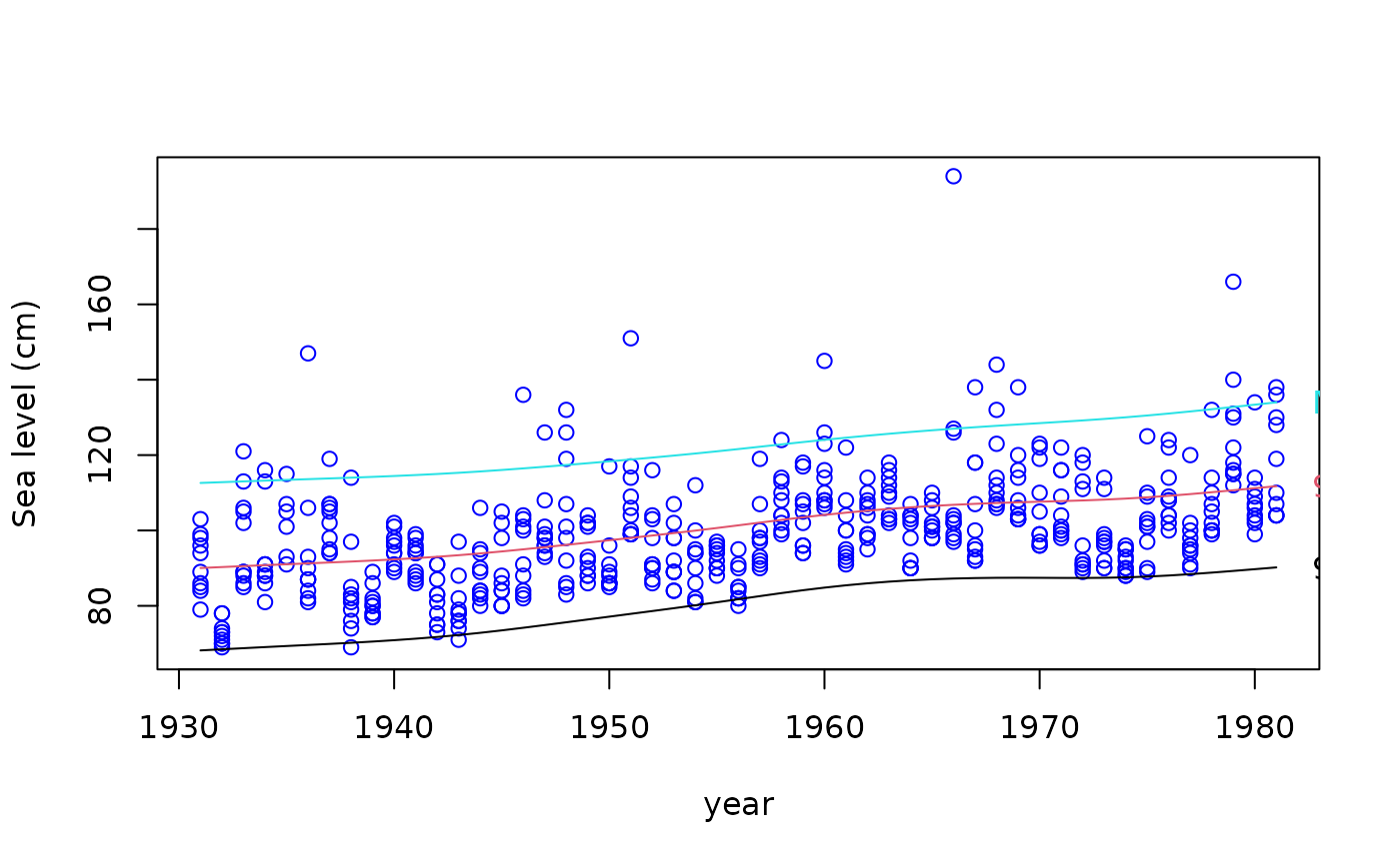
 # Quantile plot --- plots all the fitted values
qtplot(fit3, mpv = TRUE, lcol = c(1, 2, 5), tcol = c(1, 2, 5), lwd = 2,
pcol = "blue", tadj = 0.1, ylab = "Sea level (cm)")
# Quantile plot --- plots all the fitted values
qtplot(fit3, mpv = TRUE, lcol = c(1, 2, 5), tcol = c(1, 2, 5), lwd = 2,
pcol = "blue", tadj = 0.1, ylab = "Sea level (cm)")
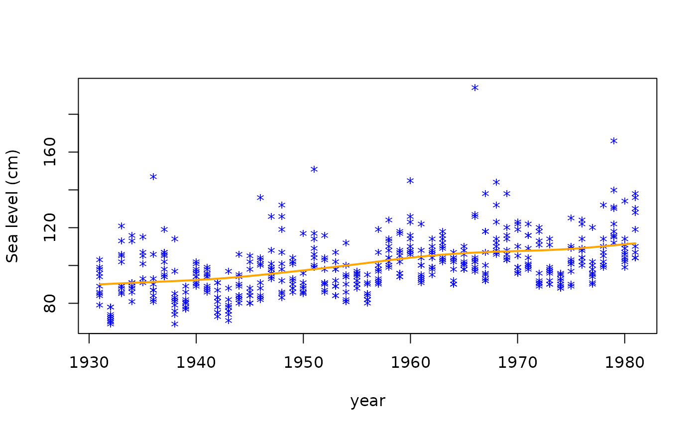
 # Plot the 99 percentile only
year <- venice[["year"]]
matplot(year, Y, ylab = "Sea level (cm)", type = "n")
matpoints(year, Y, pch = "*", col = "blue")
lines(year, fitted(fit3)[, "99%"], lwd = 2, col = "orange")
# Plot the 99 percentile only
year <- venice[["year"]]
matplot(year, Y, ylab = "Sea level (cm)", type = "n")
matpoints(year, Y, pch = "*", col = "blue")
lines(year, fitted(fit3)[, "99%"], lwd = 2, col = "orange")
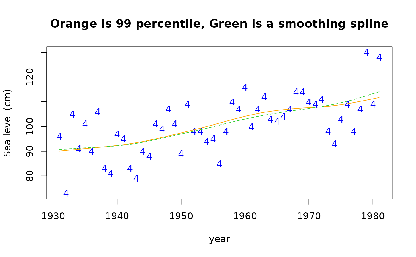
 # Check the 99 percentiles with a smoothing spline.
# Nb. (1-0.99) * 365 = 3.65 is approx. 4, meaning the 4th order
# statistic is approximately the 99 percentile.
plot(year, Y[, 4], ylab = "Sea level (cm)", type = "n",
main = "Orange is 99 percentile, Green is a smoothing spline")
points(year, Y[, 4], pch = "4", col = "blue")
lines(year, fitted(fit3)[, "99%"], lty = 1, col = "orange")
lines(smooth.spline(year, Y[, 4], df = 4), col = "limegreen", lty = 2)
# Check the 99 percentiles with a smoothing spline.
# Nb. (1-0.99) * 365 = 3.65 is approx. 4, meaning the 4th order
# statistic is approximately the 99 percentile.
plot(year, Y[, 4], ylab = "Sea level (cm)", type = "n",
main = "Orange is 99 percentile, Green is a smoothing spline")
points(year, Y[, 4], pch = "4", col = "blue")
lines(year, fitted(fit3)[, "99%"], lty = 1, col = "orange")
lines(smooth.spline(year, Y[, 4], df = 4), col = "limegreen", lty = 2)
 # \dontrun{}