Probit Link Function

Computes the probit transformation, including its inverse and the first two derivatives.

probitlink(theta, bvalue = NULL, inverse = FALSE, deriv = 0,
           short = TRUE, tag = FALSE)

Arguments

theta

Numeric or character. See below for further details.

bvalue

See Links.

inverse, deriv, short, tag

Details at Links.

Details

The probit link function is commonly used for parameters that lie in the unit interval. It is the inverse CDF of the standard normal distribution. Numerical values of theta close to 0 or 1 or out of range result in Inf, -Inf, NA or NaN.

Value

For deriv = 0, the probit of theta, i.e., qnorm(theta) when inverse = FALSE, and if inverse = TRUE then pnorm(theta).

For deriv = 1, then the function returns d eta / d theta as a function of theta if inverse = FALSE, else if inverse = TRUE then it returns the reciprocal.

References

McCullagh, P. and Nelder, J. A. (1989). Generalized Linear Models, 2nd ed. London: Chapman & Hall.

Author

Thomas W. Yee

Note

Numerical instability may occur when theta is close to 1 or 0. One way of overcoming this is to use bvalue.

In terms of the threshold approach with cumulative probabilities for an ordinal response this link function corresponds to the univariate normal distribution (see uninormal).

See also

Links, logitlink, clogloglink, cauchitlink, Normal.

Examples

p <- seq(0.01, 0.99, by = 0.01)
probitlink(p)
#>  [1] -2.32634787 -2.05374891 -1.88079361 -1.75068607 -1.64485363 -1.55477359
#>  [7] -1.47579103 -1.40507156 -1.34075503 -1.28155157 -1.22652812 -1.17498679
#> [13] -1.12639113 -1.08031934 -1.03643339 -0.99445788 -0.95416525 -0.91536509
#> [19] -0.87789630 -0.84162123 -0.80642125 -0.77219321 -0.73884685 -0.70630256
#> [25] -0.67448975 -0.64334541 -0.61281299 -0.58284151 -0.55338472 -0.52440051
#> [31] -0.49585035 -0.46769880 -0.43991317 -0.41246313 -0.38532047 -0.35845879
#> [37] -0.33185335 -0.30548079 -0.27931903 -0.25334710 -0.22754498 -0.20189348
#> [43] -0.17637416 -0.15096922 -0.12566135 -0.10043372 -0.07526986 -0.05015358
#> [49] -0.02506891  0.00000000  0.02506891  0.05015358  0.07526986  0.10043372
#> [55]  0.12566135  0.15096922  0.17637416  0.20189348  0.22754498  0.25334710
#> [61]  0.27931903  0.30548079  0.33185335  0.35845879  0.38532047  0.41246313
#> [67]  0.43991317  0.46769880  0.49585035  0.52440051  0.55338472  0.58284151
#> [73]  0.61281299  0.64334541  0.67448975  0.70630256  0.73884685  0.77219321
#> [79]  0.80642125  0.84162123  0.87789630  0.91536509  0.95416525  0.99445788
#> [85]  1.03643339  1.08031934  1.12639113  1.17498679  1.22652812  1.28155157
#> [91]  1.34075503  1.40507156  1.47579103  1.55477359  1.64485363  1.75068607
#> [97]  1.88079361  2.05374891  2.32634787
max(abs(probitlink(probitlink(p), inverse = TRUE) - p))  # Should be 0
#> [1] 1.110223e-16

p <- c(seq(-0.02, 0.02, by = 0.01), seq(0.97, 1.02, by = 0.01))
probitlink(p)  # Has NAs
#>  [1]       NaN       NaN      -Inf -2.326348 -2.053749  1.880794  2.053749
#>  [8]  2.326348       Inf       NaN       NaN
probitlink(p, bvalue = .Machine$double.eps)  # Has no NAs
#>  [1] -8.125891 -8.125891 -8.125891 -2.326348 -2.053749  1.880794  2.053749
#>  [8]  2.326348  8.125891  8.125891  8.125891

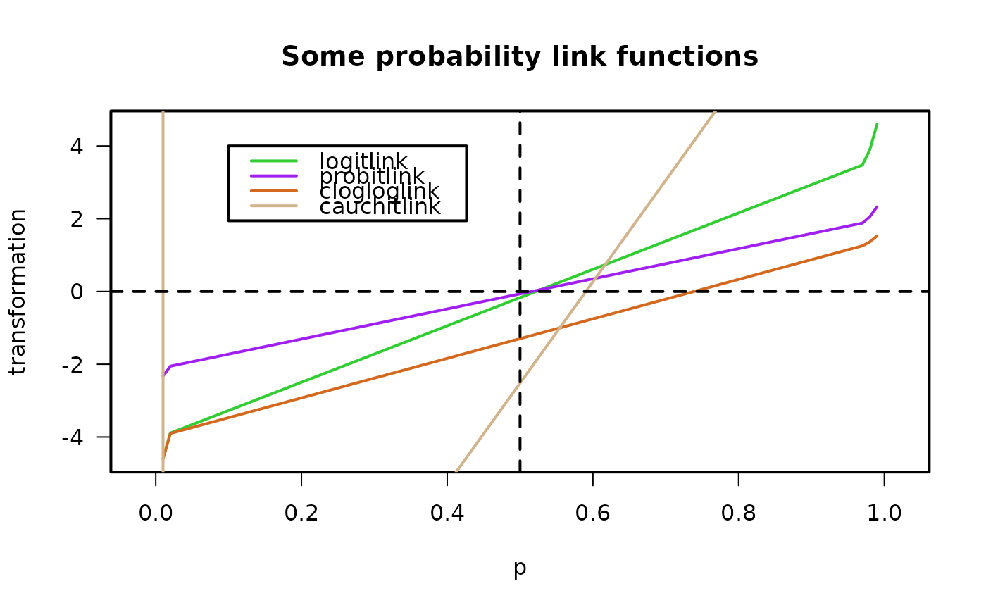
if (FALSE) p <- seq(0.01, 0.99, by = 0.01); par(lwd = (mylwd <- 2))
plot(p, logitlink(p), type = "l", col = "limegreen", ylab = "transformation",
     las = 1, main = "Some probability link functions")
lines(p,  probitlink(p), col = "purple")
lines(p, clogloglink(p), col = "chocolate")
lines(p, cauchitlink(p), col = "tan")
abline(v = 0.5, h = 0, lty = "dashed")
legend(0.1, 4, c("logitlink", "probitlink", "clogloglink", "cauchitlink"),
       col = c("limegreen", "purple", "chocolate", "tan"), lwd = mylwd)

par(lwd = 1)  # \dontrun{}