Mixture of Two Poisson Distributions

Estimates the three parameters of a mixture of two Poisson distributions by maximum likelihood estimation.

mix2poisson(lphi = "logitlink", llambda = "loglink",
            iphi = 0.5, il1 = NULL, il2 = NULL,
            qmu = c(0.2, 0.8), nsimEIM = 100, zero = "phi")

Arguments

lphi, llambda

Link functions for the parameter $\phi$ and $\lambda$. See Links for more choices.

iphi

Initial value for $\phi$, whose value must lie between 0 and 1.

il1, il2

Optional initial value for $\lambda_1$ and $\lambda_2$. These values must be positive. The default is to compute initial values internally using the argument qmu.

qmu

Vector with two values giving the probabilities relating to the sample quantiles for obtaining initial values for $\lambda_1$ and $\lambda_2$. The two values are fed in as the probs argument into quantile.

nsimEIM, zero

See CommonVGAMffArguments.

Details

The probability function can be loosely written as $$P(Y=y) = \phi \, Poisson(\lambda_1) + (1-\phi) \, Poisson(\lambda_2)$$ where $\phi$ is the probability an observation belongs to the first group, and $y=0,1,2,\ldots$. The parameter $\phi$ satisfies $0 < \phi < 1$. The mean of $Y$ is $\phi\lambda_1+(1-\phi)\lambda_2$ and this is returned as the fitted values. By default, the three linear/additive predictors are $(logit(\phi), \log(\lambda_1), \log(\lambda_2))^T$.

Value

An object of class "vglmff" (see vglmff-class). The object is used by modelling functions such as vglm and vgam.

Warning

This VGAM family function requires care for a successful application. In particular, good initial values are required because of the presence of local solutions. Therefore running this function with several different combinations of arguments such as iphi, il1, il2, qmu is highly recommended. Graphical methods such as hist can be used as an aid.

With grouped data (i.e., using the weights argument) one has to use a large value of nsimEIM; see the example below.

This VGAM family function is experimental and should be used with care.

Author

T. W. Yee

Note

The response must be integer-valued since dpois is invoked.

Fitting this model successfully to data can be difficult due to local solutions and ill-conditioned data. It pays to fit the model several times with different initial values, and check that the best fit looks reasonable. Plotting the results is recommended. This function works better as $\lambda_1$ and $\lambda_2$ become more different. The default control argument trace = TRUE is to encourage monitoring convergence.

Examples

if (FALSE)  # Example 1: simulated data
nn <- 1000
mu1 <- exp(2.5)  # Also known as lambda1
mu2 <- exp(3)
(phi <- logitlink(-0.5, inverse = TRUE))
#> [1] 0.3775407
mdata <- data.frame(y = rpois(nn, ifelse(runif(nn) < phi, mu1, mu2)))
mfit <- vglm(y ~ 1, mix2poisson, data = mdata)
#> Iteration 1: loglikelihood = -1575.8839
#> Iteration 2: loglikelihood = -1575.6883
#> Iteration 3: loglikelihood = -1575.6868
#> Iteration 4: loglikelihood = -1575.6868
#> Iteration 5: loglikelihood = -1575.6868
coef(mfit, matrix = TRUE)
#>             logitlink(phi) loglink(lambda1) loglink(lambda2)
#> (Intercept)     -0.4095453         2.515517          3.01773

# Compare the results with the truth
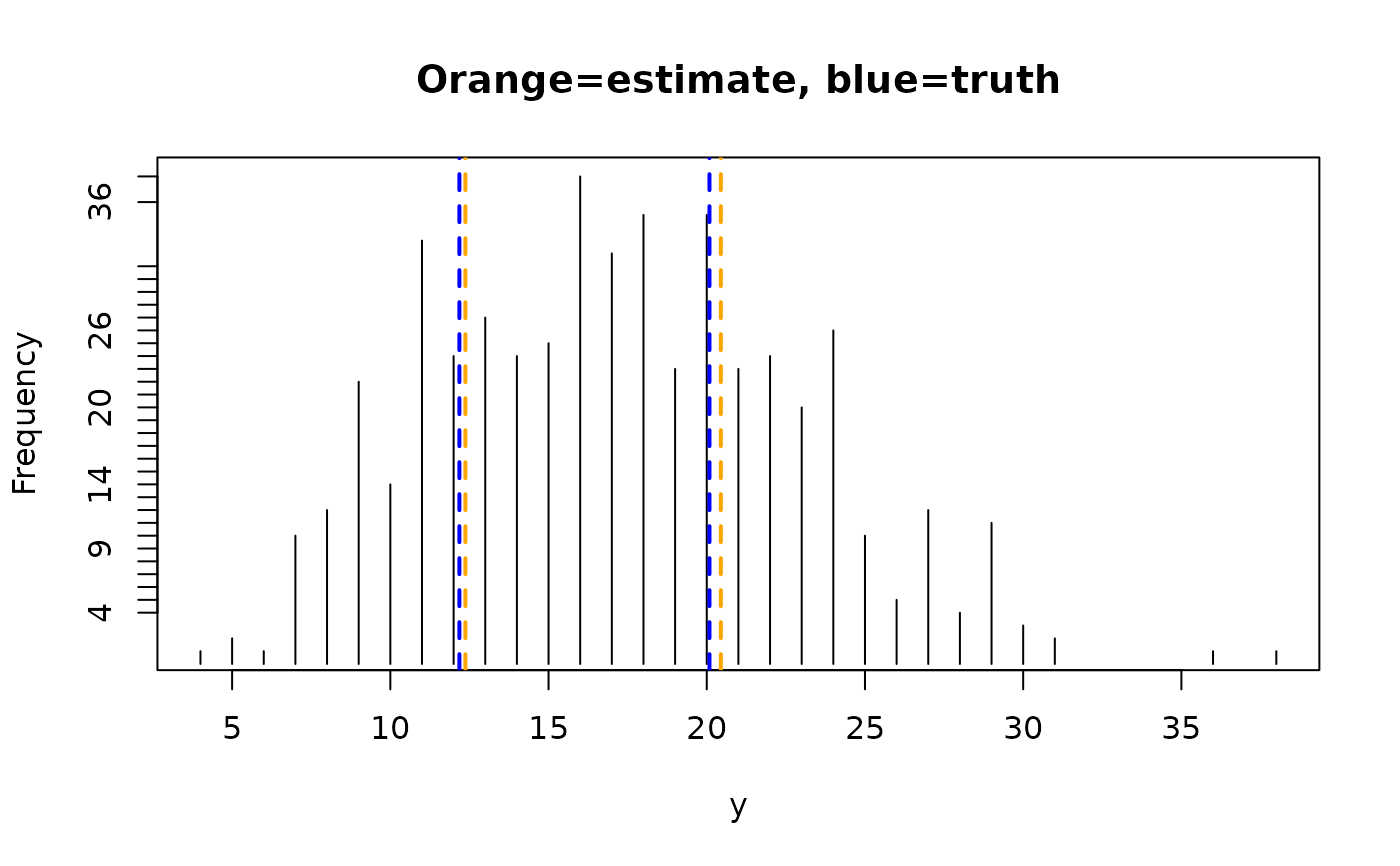
round(rbind('Estimated' = Coef(mfit), 'Truth' = c(phi, mu1, mu2)), 2)
#>            phi lambda1 lambda2
#> Estimated 0.40   12.37   20.44
#> Truth     0.38   12.18   20.09

ty <- with(mdata, table(y))
plot(names(ty), ty, type = "h", main = "Orange=estimate, blue=truth",
     ylab = "Frequency", xlab = "y")
abline(v = Coef(mfit)[-1], lty = 2, col = "orange", lwd = 2)
abline(v = c(mu1, mu2), lty = 2, col = "blue", lwd = 2)


# Example 2: London Times data (Lange, 1997, p.31)
ltdata1 <- data.frame(deaths = 0:9,
                      freq = c(162,267,271, 185,111,61,27,8,3,1))
ltdata2 <- data.frame(y = with(ltdata1, rep(deaths, freq)))

# Usually this does not work well unless nsimEIM is large
Mfit <- vglm(deaths ~ 1, weight = freq, data = ltdata1,
        mix2poisson(iphi=0.3, il1=1, il2=2.5, nsimEIM=5000))
#> Iteration 1: loglikelihood = -1989.9835
#> Applying Greenstadt modification to 10 matrices
#> Iteration 2: loglikelihood = -1993.7258
#> Taking a modified step..
#> Iteration  2 :  loglikelihood = -1989.9756
#> Iteration 3: loglikelihood = -1989.9536
#> Iteration 4: loglikelihood = -1989.9575
#> Taking a modified step.
#> Iteration  4 :  loglikelihood = -1989.9469
#> Iteration 5: loglikelihood = -1989.9459
#> Iteration 6: loglikelihood = -1989.9459

# This works better in general
Mfit = vglm(y ~ 1, mix2poisson(iphi=0.3, il1=1, il2=2.5), ltdata2)
#> Iteration 1: loglikelihood = -1990.00277
#> Iteration 2: loglikelihood = -1989.94587
#> Iteration 3: loglikelihood = -1989.94586
#> Iteration 4: loglikelihood = -1989.94586
coef(Mfit, matrix = TRUE)
#>             logitlink(phi) loglink(lambda1) loglink(lambda2)
#> (Intercept)     -0.5758701        0.2280049        0.9796043
Coef(Mfit)
#>       phi   lambda1   lambda2 
#> 0.3598834 1.2560915 2.6634020 
 # \dontrun{}