Nakagami Regression Family Function

Estimation of the two parameters of the Nakagami distribution by maximum likelihood estimation.

nakagami(lscale = "loglink", lshape = "loglink", iscale = 1,
         ishape = NULL, nowarning = FALSE, zero = "shape")

Arguments

nowarning

Logical. Suppress a warning?

lscale, lshape

Parameter link functions applied to the scale and shape parameters. Log links ensure they are positive. See Links for more choices and information.

iscale, ishape

Optional initial values for the shape and scale parameters. For ishape, a NULL value means it is obtained in the initialize slot based on the value of iscale. For iscale, assigning a NULL means a value is obtained in the initialize slot, however, setting another numerical value is recommended if convergence fails or is too slow.

zero

See CommonVGAMffArguments.

Details

The Nakagami distribution, which is useful for modelling wireless systems such as radio links, can be written $$f(y) = 2 (shape/scale)^{shape} y^{2 \times shape-1} \exp(-shape \times y^2/scale) / \Gamma(shape)$$ for $y > 0$, $shape > 0$, $scale > 0$. The mean of $Y$ is $\sqrt{scale/shape} \times \Gamma(shape+0.5) / \Gamma(shape)$ and these are returned as the fitted values. By default, the linear/additive predictors are $\eta_1=\log(scale)$ and $\eta_2=\log(shape)$. Fisher scoring is implemented.

Value

An object of class "vglmff" (see vglmff-class). The object is used by modelling functions such as vglm, and vgam.

References

Nakagami, M. (1960). The m-distribution: a general formula of intensity distribution of rapid fading, pp.3–36 in: Statistical Methods in Radio Wave Propagation. W. C. Hoffman, Ed., New York: Pergamon.

Author

T. W. Yee

Note

The Nakagami distribution is also known as the Nakagami-m distribution, where $m=shape$ here. Special cases: $m=0.5$ is a one-sided Gaussian distribution and $m=1$ is a Rayleigh distribution. The second moment is $E(Y^2)=m$.

If $Y$ has a Nakagami distribution with parameters shape and scale then $Y^2$ has a gamma distribution with shape parameter shape and scale parameter scale/shape.

Examples

nn <- 1000; shape <- exp(0); Scale <- exp(1)
ndata <- data.frame(y1 = sqrt(rgamma(nn, shape = shape, scale = Scale/shape)))
nfit <- vglm(y1 ~ 1, nakagami, data = ndata, trace = TRUE, crit = "coef")
#> Iteration 1: coefficients = -0.31044169, -3.05663287
#> Iteration 2: coefficients =  2.3690544, -2.2329295
#> Iteration 3: coefficients =  1.6214594, -1.4901743
#> Iteration 4: coefficients =  1.1545173, -0.8273739
#> Iteration 5: coefficients =  1.00480273, -0.30940127
#> Iteration 6: coefficients =  0.992411533, -0.053945349
#> Iteration 7: coefficients =  0.9923341245, -0.0063795176
#> Iteration 8: coefficients =  0.9923341215, -0.0049948467
#> Iteration 9: coefficients =  0.9923341215, -0.0049937167
#> Iteration 10: coefficients =  0.9923341215, -0.0049937167
ndata <- transform(ndata, y2 = rnaka(nn, scale = Scale, shape = shape))
nfit <- vglm(y2 ~ 1, nakagami(iscale = 3), data = ndata, trace = TRUE)
#> Iteration 1: loglikelihood = -7785.1726
#> Iteration 2: loglikelihood = -6790.5897
#> Iteration 3: loglikelihood = -5803.2354
#> Iteration 4: loglikelihood = -4832.0756
#> Iteration 5: loglikelihood = -3895.1864
#> Iteration 6: loglikelihood = -3025.0533
#> Iteration 7: loglikelihood = -2269.9124
#> Iteration 8: loglikelihood = -1683.4457
#> Iteration 9: loglikelihood = -1305.739
#> Iteration 10: loglikelihood = -1140.0799
#> Iteration 11: loglikelihood = -1109.2444
#> Iteration 12: loglikelihood = -1108.2362
#> Iteration 13: loglikelihood = -1108.2351
#> Iteration 14: loglikelihood = -1108.2351
head(fitted(nfit))
#>          [,1]
#> [1,] 1.497823
#> [2,] 1.497823
#> [3,] 1.497823
#> [4,] 1.497823
#> [5,] 1.497823
#> [6,] 1.497823
with(ndata, mean(y2))
#> [1] 1.493996
coef(nfit, matrix = TRUE)
#>             loglink(scale) loglink(shape)
#> (Intercept)       1.043427     0.02741628
(Cfit <- Coef(nfit))
#>    scale    shape 
#> 2.838930 1.027796 
if (FALSE)  sy <- with(ndata, sort(y2))
hist(with(ndata, y2), prob = TRUE, main = "", xlab = "y", ylim = c(0, 0.6),
     col = "lightblue")

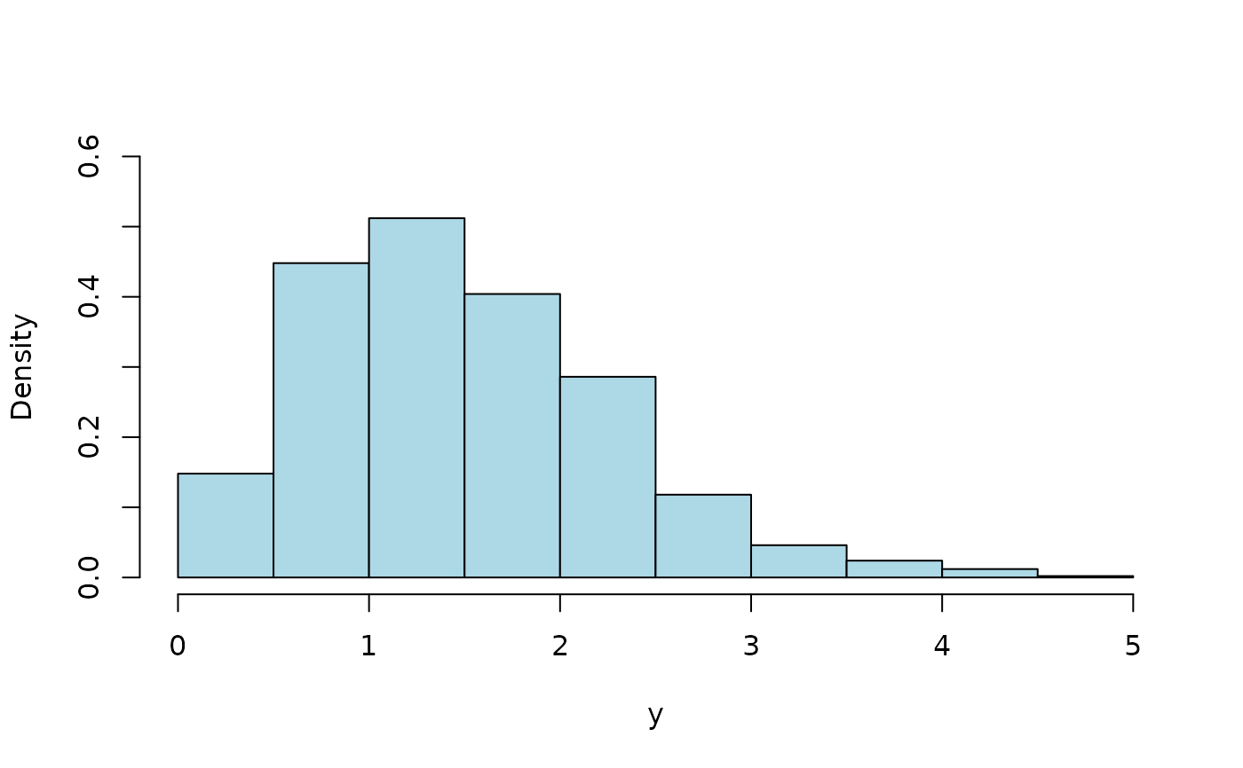lines(dnaka(sy, scale = Cfit["scale"], shape = Cfit["shape"]) ~ sy,
      data = ndata, col = "orange")  # \dontrun{}
#> Error in eval(predvars, data, env): object 'sy' not found