Tobit Regression
tobit.RdFits a Tobit regression model.
tobit(Lower = 0, Upper = Inf, lmu = "identitylink",
      lsd = "loglink", imu = NULL, isd = NULL,
      type.fitted = c("uncensored", "censored", "mean.obs"),
      byrow.arg = FALSE, imethod = 1, zero = "sd")
Arguments
- Lower
Numeric. It is the value \(L\) described below. Any value of the linear model \(x_i^T \beta\) that is less than this lowerbound is assigned this value. Hence this should be the smallest possible value in the response variable. May be a vector (see below for more information).
- Upper
Numeric. It is the value \(U\) described below. Any value of the linear model \(x_i^T \beta\) that is greater than this upperbound is assigned this value. Hence this should be the largest possible value in the response variable. May be a vector (see below for more information).
- lmu, lsd
Parameter link functions for the mean and standard deviation parameters. See
Linksfor more choices. The standard deviation is a positive quantity, therefore a log link is its default.- imu, isd, byrow.arg
See
CommonVGAMffArgumentsfor information.- type.fitted
Type of fitted value returned. The first choice is default and is the ordinary uncensored or unbounded linear model. If
"censored"then the fitted values in the interval \([L, U]\). If"mean.obs"then the mean of the observations is returned; this is a doubly truncated normal distribution augmented by point masses at the truncation points (seedtobit). SeeCommonVGAMffArgumentsfor more information.- imethod
Initialization method. Either 1 or 2 or 3, this specifies some methods for obtaining initial values for the parameters. See
CommonVGAMffArgumentsfor information.- zero
A vector, e.g., containing the value 1 or 2. If so, the mean or standard deviation respectively are modelled as an intercept-only. Setting
zero = NULLmeans both linear/additive predictors are modelled as functions of the explanatory variables. SeeCommonVGAMffArgumentsfor more information.
Details
The Tobit model can be written $$y_i^* = x_i^T \beta + \varepsilon_i$$ where the \(e_i \sim N(0,\sigma^2)\) independently and \(i=1,\ldots,n\). However, we measure \(y_i = y_i^*\) only if \(y_i^* > L\) and \(y_i^* < U\) for some cutpoints \(L\) and \(U\). Otherwise we let \(y_i=L\) or \(y_i=U\), whatever is closer. The Tobit model is thus a multiple linear regression but with censored responses if it is below or above certain cutpoints.
The defaults for Lower and Upper and
lmu correspond to the standard Tobit model.
Fisher scoring is used for the standard and nonstandard
models.
By default, the mean \(x_i^T \beta\) is
the first linear/additive predictor, and the log of
the standard deviation is the second linear/additive
predictor. The Fisher information matrix for uncensored
data is diagonal. The fitted values are the estimates
of \(x_i^T \beta\).
Warning
If values of the response and Lower and/or Upper
are not integers then there is the danger that the value is
wrongly interpreted as uncensored.
For example, if the first 10 values of the response were
runif(10) and Lower was assigned these value then
testing y[1:10] == Lower[1:10] is numerically fraught.
Currently, if any y < Lower or y > Upper then
a warning is issued.
The function round2 may be useful.
Value
An object of class "vglmff"
(see vglmff-class).
The object is used by modelling functions
such as vglm,
and vgam.
References
Tobin, J. (1958). Estimation of relationships for limited dependent variables. Econometrica 26, 24–36.
Note
The response can be a matrix.
If so, then Lower and Upper
are recycled into a matrix with the number of columns equal
to the number of responses,
and the recycling is done row-wise if
byrow.arg = TRUE.
The default order is as matrix, which
is byrow.arg = FALSE.
For example, these are returned in fit4@misc$Lower and
fit4@misc$Upper below.
If there is no censoring then
uninormal is recommended instead.
Any value of the
response less than Lower or greater
than Upper will
be assigned the value Lower and Upper
respectively,
and a warning will be issued.
The fitted object has components censoredL
and censoredU
in the extra slot which specifies whether
observations
are censored in that direction.
The function cens.normal is an alternative
to tobit().
When obtaining initial values, if the algorithm would otherwise want to fit an underdetermined system of equations, then it uses the entire data set instead. This might result in rather poor quality initial values, and consequently, monitoring convergence is advised.
See also
Examples
# Here, fit1 is a standard Tobit model and fit2 is nonstandard
tdata <- data.frame(x2 = seq(-1, 1, length = (nn <- 100)))
set.seed(1)
Lower <- 1; Upper <- 4 # For the nonstandard Tobit model
tdata <- transform(tdata,
Lower.vec = rnorm(nn, Lower, 0.5),
Upper.vec = rnorm(nn, Upper, 0.5))
meanfun1 <- function(x) 0 + 2*x
meanfun2 <- function(x) 2 + 2*x
meanfun3 <- function(x) 3 + 2*x
tdata <- transform(tdata,
y1 = rtobit(nn, mean = meanfun1(x2)), # Standard Tobit model
y2 = rtobit(nn, mean = meanfun2(x2), Lower = Lower, Upper = Upper),
y3 = rtobit(nn, mean = meanfun3(x2), Lower = Lower.vec,
Upper = Upper.vec),
y4 = rtobit(nn, mean = meanfun3(x2), Lower = Lower.vec,
Upper = Upper.vec))
with(tdata, table(y1 == 0)) # How many censored values?
#>
#> FALSE TRUE
#> 52 48
with(tdata, table(y2 == Lower | y2 == Upper)) # Ditto
#>
#> FALSE TRUE
#> 66 34
with(tdata, table(attr(y2, "cenL")))
#>
#> FALSE TRUE
#> 75 25
with(tdata, table(attr(y2, "cenU")))
#>
#> FALSE TRUE
#> 91 9
fit1 <- vglm(y1 ~ x2, tobit, data = tdata, trace = TRUE)
#> Iteration 1: loglikelihood = -94.952489
#> Iteration 2: loglikelihood = -90.601839
#> Iteration 3: loglikelihood = -90.335693
#> Iteration 4: loglikelihood = -90.334971
#> Iteration 5: loglikelihood = -90.334971
coef(fit1, matrix = TRUE)
#> mu loglink(sd)
#> (Intercept) 0.06794616 -0.06234739
#> x2 2.02595920 0.00000000
summary(fit1)
#>
#> Call:
#> vglm(formula = y1 ~ x2, family = tobit, data = tdata, trace = TRUE)
#>
#> Coefficients:
#> Estimate Std. Error z value Pr(>|z|)
#> (Intercept):1 0.06795 0.13614 0.499 0.618
#> (Intercept):2 -0.06235 0.10273 -0.607 0.544
#> x2 2.02596 0.23949 8.459 <2e-16 ***
#> ---
#> Signif. codes: 0 ‘***’ 0.001 ‘**’ 0.01 ‘*’ 0.05 ‘.’ 0.1 ‘ ’ 1
#>
#> Names of linear predictors: mu, loglink(sd)
#>
#> Log-likelihood: -90.335 on 197 degrees of freedom
#>
#> Number of Fisher scoring iterations: 5
#>
#> No Hauck-Donner effect found in any of the estimates
#>
fit2 <- vglm(y2 ~ x2,
tobit(Lower = Lower, Upper = Upper, type.f = "cens"),
data = tdata, trace = TRUE)
#> Iteration 1: loglikelihood = -117.40947
#> Iteration 2: loglikelihood = -115.71547
#> Iteration 3: loglikelihood = -115.66898
#> Iteration 4: loglikelihood = -115.66819
#> Iteration 5: loglikelihood = -115.66818
#> Iteration 6: loglikelihood = -115.66818
table(fit2@extra$censoredL)
#>
#> FALSE TRUE
#> 75 25
table(fit2@extra$censoredU)
#>
#> FALSE TRUE
#> 91 9
coef(fit2, matrix = TRUE)
#> mu loglink(sd)
#> (Intercept) 2.053261 -0.04893087
#> x2 1.880404 0.00000000
fit3 <- vglm(y3 ~ x2, tobit(Lower = with(tdata, Lower.vec),
Upper = with(tdata, Upper.vec),
type.f = "cens"),
data = tdata, trace = TRUE)
#> Iteration 1: loglikelihood = -118.69013
#> Iteration 2: loglikelihood = -117.11926
#> Iteration 3: loglikelihood = -117.07583
#> Iteration 4: loglikelihood = -117.07438
#> Iteration 5: loglikelihood = -117.07433
#> Iteration 6: loglikelihood = -117.07433
#> Iteration 7: loglikelihood = -117.07433
table(fit3@extra$censoredL)
#>
#> FALSE TRUE
#> 84 16
table(fit3@extra$censoredU)
#>
#> FALSE TRUE
#> 77 23
coef(fit3, matrix = TRUE)
#> mu loglink(sd)
#> (Intercept) 2.904743 0.09173307
#> x2 2.178193 0.00000000
# fit4 is fit3 but with type.fitted = "uncen".
fit4 <- vglm(cbind(y3, y4) ~ x2,
tobit(Lower = rep(with(tdata, Lower.vec), each = 2),
Upper = rep(with(tdata, Upper.vec), each = 2),
byrow.arg = TRUE),
data = tdata, crit = "coeff", trace = TRUE)
#> Iteration 1: coefficients =
#> 2.89014257, 0.25304478, 2.96031053, 0.20508806, 2.12538698, 2.02573207
#> Iteration 2: coefficients =
#> 2.885765205, 0.093423424, 2.942093302, 0.043317927, 2.232760342, 2.239483502
#> Iteration 3: coefficients =
#> 2.905736069, 0.096906039, 2.951169180, 0.023582998, 2.181484799, 2.175403035
#> Iteration 4: coefficients =
#> 2.904410822, 0.091524289, 2.950632485, 0.016355913, 2.179996601, 2.164449979
#> Iteration 5: coefficients =
#> 2.904781633, 0.091888984, 2.950534264, 0.014991137, 2.178221623, 2.160988668
#> Iteration 6: coefficients =
#> 2.904730135, 0.091715330, 2.950515287, 0.014622934, 2.178246473, 2.160270160
#> Iteration 7: coefficients =
#> 2.904742983, 0.091733074, 2.950510499, 0.014541499, 2.178193053, 2.160085708
#> Iteration 8: coefficients =
#> 2.904740949, 0.091727259, 2.950509419, 0.014521425, 2.178195929, 2.160043739
#> Iteration 9: coefficients =
#> 2.904741408, 0.091728014, 2.950509157, 0.014516762, 2.178194244, 2.160033552
#> Iteration 10: coefficients =
#> 2.904741329, 0.091727813, 2.950509096, 0.014515643, 2.178194396, 2.160031165
#> Iteration 11: coefficients =
#> 2.904741346, 0.091727843, 2.950509081, 0.014515379, 2.178194341, 2.160030595
#> Iteration 12: coefficients =
#> 2.904741343, 0.091727836, 2.950509078, 0.014515317, 2.178194347, 2.160030461
#> Iteration 13: coefficients =
#> 2.904741344, 0.091727837, 2.950509077, 0.014515302, 2.178194345, 2.160030429
#> Iteration 14: coefficients =
#> 2.904741344, 0.091727837, 2.950509077, 0.014515298, 2.178194346, 2.160030421
#> Iteration 15: coefficients =
#> 2.904741344, 0.091727837, 2.950509077, 0.014515297, 2.178194346, 2.160030419
head(fit4@extra$censoredL) # A matrix
#> y3 y4
#> 1 FALSE FALSE
#> 2 FALSE TRUE
#> 3 TRUE TRUE
#> 4 TRUE TRUE
#> 5 TRUE FALSE
#> 6 FALSE FALSE
head(fit4@extra$censoredU) # A matrix
#> y3 y4
#> 1 FALSE FALSE
#> 2 FALSE FALSE
#> 3 FALSE FALSE
#> 4 FALSE FALSE
#> 5 FALSE FALSE
#> 6 FALSE FALSE
head(fit4@misc$Lower) # A matrix
#> [,1] [,2]
#> [1,] 0.6867731 0.6867731
#> [2,] 1.0918217 1.0918217
#> [3,] 0.5821857 0.5821857
#> [4,] 1.7976404 1.7976404
#> [5,] 1.1647539 1.1647539
#> [6,] 0.5897658 0.5897658
head(fit4@misc$Upper) # A matrix
#> [,1] [,2]
#> [1,] 3.689817 3.689817
#> [2,] 4.021058 4.021058
#> [3,] 3.544539 3.544539
#> [4,] 4.079014 4.079014
#> [5,] 3.672708 3.672708
#> [6,] 4.883644 4.883644
coef(fit4, matrix = TRUE)
#> mu1 loglink(sd1) mu2 loglink(sd2)
#> (Intercept) 2.904741 0.09172784 2.950509 0.0145153
#> x2 2.178194 0.00000000 2.160030 0.0000000
if (FALSE) # Plot fit1--fit4
par(mfrow = c(2, 2))
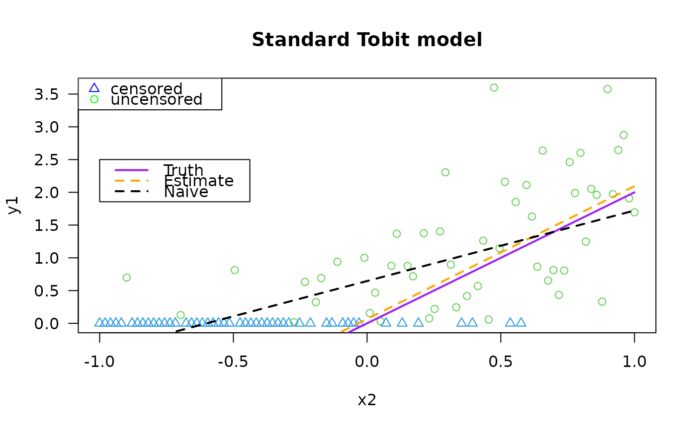
plot(y1 ~ x2, tdata, las = 1, main = "Standard Tobit model",
col = as.numeric(attr(y1, "cenL")) + 3,
pch = as.numeric(attr(y1, "cenL")) + 1)
legend(x = "topleft", leg = c("censored", "uncensored"),
pch = c(2, 1), col = c("blue", "green"))
legend(-1.0, 2.5, c("Truth", "Estimate", "Naive"), lwd = 2,
col = c("purple", "orange", "black"), lty = c(1, 2, 2))
lines(meanfun1(x2) ~ x2, tdata, col = "purple", lwd = 2)
lines(fitted(fit1) ~ x2, tdata, col = "orange", lwd = 2, lty = 2)
lines(fitted(lm(y1 ~ x2, tdata)) ~ x2, tdata, col = "black",
lty = 2, lwd = 2) # This is simplest but wrong!
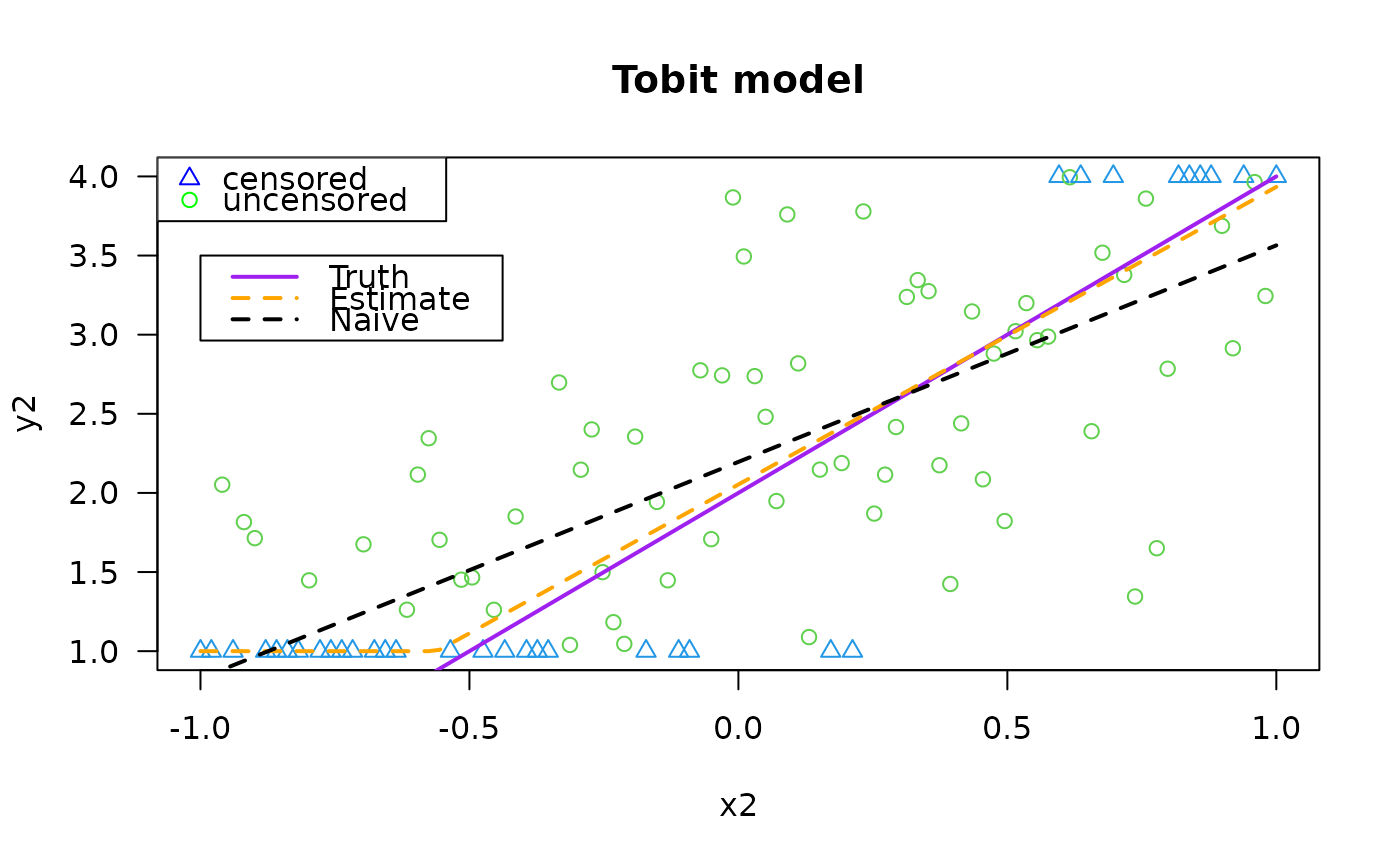
 plot(y2 ~ x2, data = tdata, las = 1, main = "Tobit model",
col = as.numeric(attr(y2, "cenL")) + 3 +
as.numeric(attr(y2, "cenU")),
pch = as.numeric(attr(y2, "cenL")) + 1 +
as.numeric(attr(y2, "cenU")))
legend(x = "topleft", leg = c("censored", "uncensored"),
pch = c(2, 1), col = c("blue", "green"))
legend(-1.0, 3.5, c("Truth", "Estimate", "Naive"), lwd = 2,
col = c("purple", "orange", "black"), lty = c(1, 2, 2))
lines(meanfun2(x2) ~ x2, tdata, col = "purple", lwd = 2)
lines(fitted(fit2) ~ x2, tdata, col = "orange", lwd = 2, lty = 2)
lines(fitted(lm(y2 ~ x2, tdata)) ~ x2, tdata, col = "black",
lty = 2, lwd = 2) # This is simplest but wrong!
plot(y2 ~ x2, data = tdata, las = 1, main = "Tobit model",
col = as.numeric(attr(y2, "cenL")) + 3 +
as.numeric(attr(y2, "cenU")),
pch = as.numeric(attr(y2, "cenL")) + 1 +
as.numeric(attr(y2, "cenU")))
legend(x = "topleft", leg = c("censored", "uncensored"),
pch = c(2, 1), col = c("blue", "green"))
legend(-1.0, 3.5, c("Truth", "Estimate", "Naive"), lwd = 2,
col = c("purple", "orange", "black"), lty = c(1, 2, 2))
lines(meanfun2(x2) ~ x2, tdata, col = "purple", lwd = 2)
lines(fitted(fit2) ~ x2, tdata, col = "orange", lwd = 2, lty = 2)
lines(fitted(lm(y2 ~ x2, tdata)) ~ x2, tdata, col = "black",
lty = 2, lwd = 2) # This is simplest but wrong!
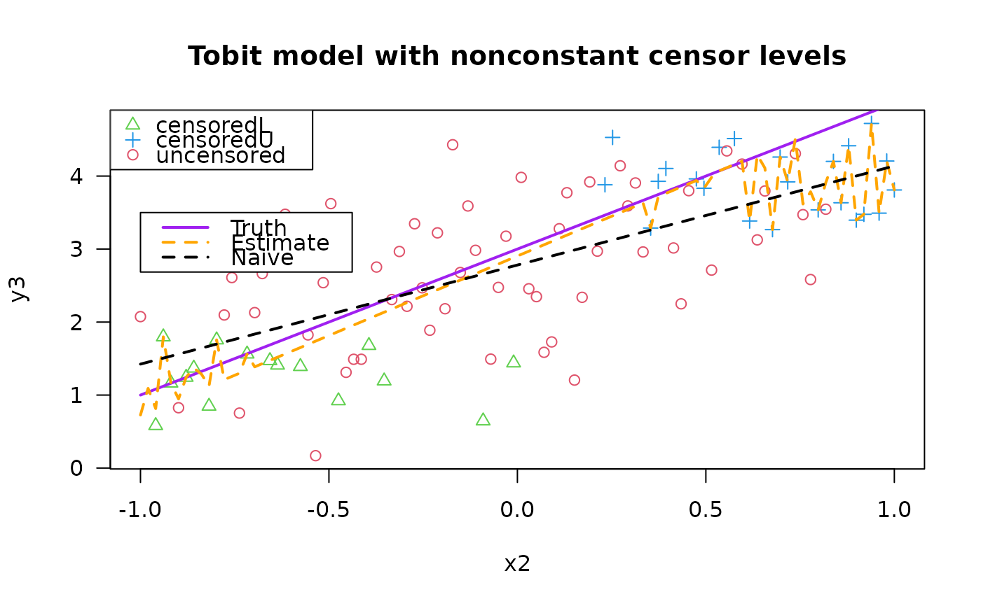
 plot(y3 ~ x2, data = tdata, las = 1,
main = "Tobit model with nonconstant censor levels",
col = as.numeric(attr(y3, "cenL")) + 2 +
as.numeric(attr(y3, "cenU") * 2),
pch = as.numeric(attr(y3, "cenL")) + 1 +
as.numeric(attr(y3, "cenU") * 2))
legend(x = "topleft", pch = c(2, 3, 1), col = c(3, 4, 2),
leg = c("censoredL", "censoredU", "uncensored"))
legend(-1.0, 3.5, c("Truth", "Estimate", "Naive"), lwd = 2,
col = c("purple", "orange", "black"), lty = c(1, 2, 2))
lines(meanfun3(x2) ~ x2, tdata, col = "purple", lwd = 2)
lines(fitted(fit3) ~ x2, tdata, col = "orange", lwd = 2, lty = 2)
lines(fitted(lm(y3 ~ x2, tdata)) ~ x2, tdata, col = "black",
lty = 2, lwd = 2) # This is simplest but wrong!
plot(y3 ~ x2, data = tdata, las = 1,
main = "Tobit model with nonconstant censor levels",
col = as.numeric(attr(y3, "cenL")) + 2 +
as.numeric(attr(y3, "cenU") * 2),
pch = as.numeric(attr(y3, "cenL")) + 1 +
as.numeric(attr(y3, "cenU") * 2))
legend(x = "topleft", pch = c(2, 3, 1), col = c(3, 4, 2),
leg = c("censoredL", "censoredU", "uncensored"))
legend(-1.0, 3.5, c("Truth", "Estimate", "Naive"), lwd = 2,
col = c("purple", "orange", "black"), lty = c(1, 2, 2))
lines(meanfun3(x2) ~ x2, tdata, col = "purple", lwd = 2)
lines(fitted(fit3) ~ x2, tdata, col = "orange", lwd = 2, lty = 2)
lines(fitted(lm(y3 ~ x2, tdata)) ~ x2, tdata, col = "black",
lty = 2, lwd = 2) # This is simplest but wrong!
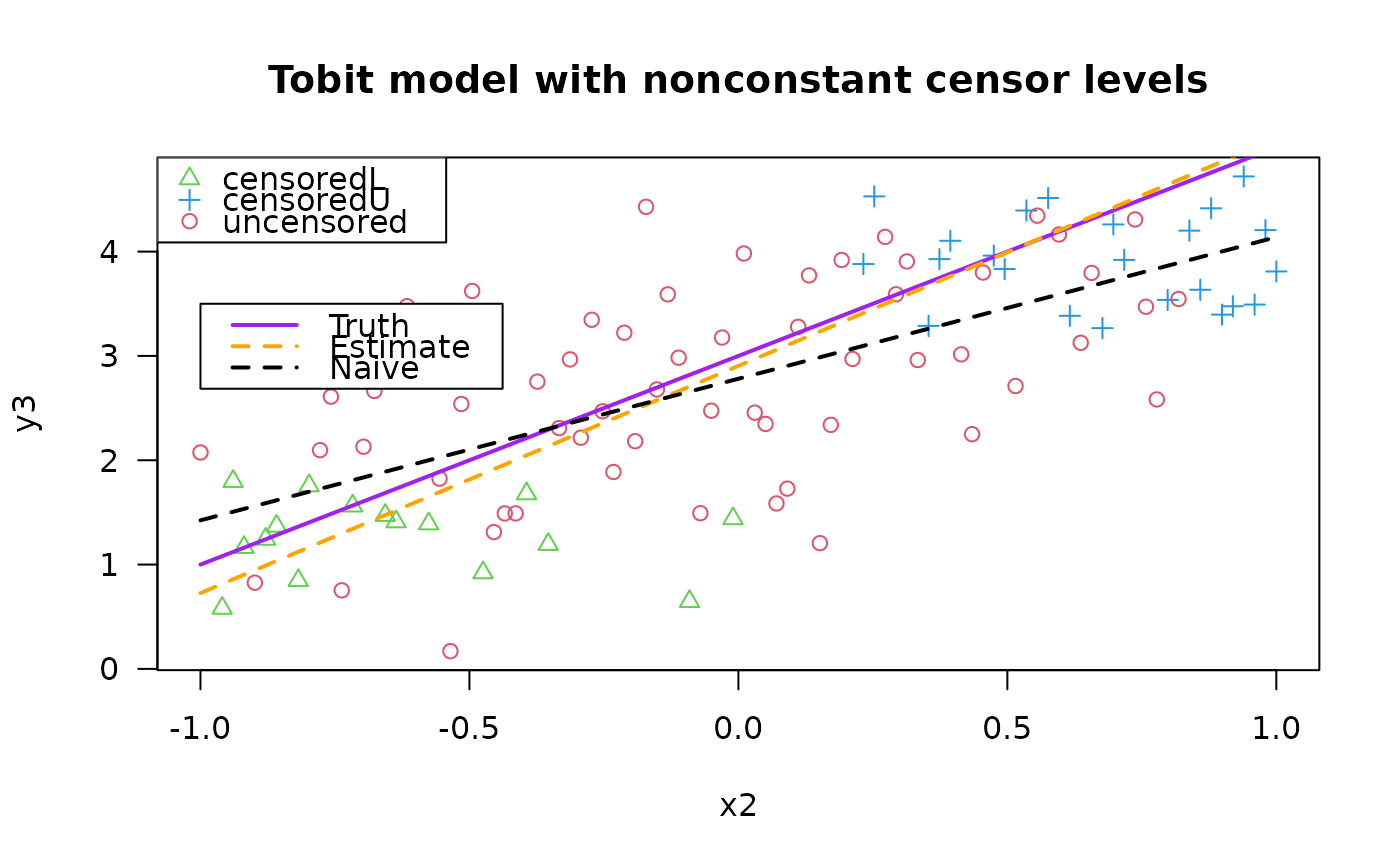
 plot(y3 ~ x2, data = tdata, las = 1,
main = "Tobit model with nonconstant censor levels",
col = as.numeric(attr(y3, "cenL")) + 2 +
as.numeric(attr(y3, "cenU") * 2),
pch = as.numeric(attr(y3, "cenL")) + 1 +
as.numeric(attr(y3, "cenU") * 2))
legend(x = "topleft", pch = c(2, 3, 1), col = c(3, 4, 2),
leg = c("censoredL", "censoredU", "uncensored"))
legend(-1.0, 3.5, c("Truth", "Estimate", "Naive"), lwd = 2,
col = c("purple", "orange", "black"), lty = c(1, 2, 2))
lines(meanfun3(x2) ~ x2, data = tdata, col = "purple", lwd = 2)
lines(fitted(fit4)[, 1] ~ x2, tdata, col="orange", lwd = 2, lty = 2)
lines(fitted(lm(y3 ~ x2, tdata)) ~ x2, data = tdata, col = "black",
lty = 2, lwd = 2) # This is simplest but wrong!
plot(y3 ~ x2, data = tdata, las = 1,
main = "Tobit model with nonconstant censor levels",
col = as.numeric(attr(y3, "cenL")) + 2 +
as.numeric(attr(y3, "cenU") * 2),
pch = as.numeric(attr(y3, "cenL")) + 1 +
as.numeric(attr(y3, "cenU") * 2))
legend(x = "topleft", pch = c(2, 3, 1), col = c(3, 4, 2),
leg = c("censoredL", "censoredU", "uncensored"))
legend(-1.0, 3.5, c("Truth", "Estimate", "Naive"), lwd = 2,
col = c("purple", "orange", "black"), lty = c(1, 2, 2))
lines(meanfun3(x2) ~ x2, data = tdata, col = "purple", lwd = 2)
lines(fitted(fit4)[, 1] ~ x2, tdata, col="orange", lwd = 2, lty = 2)
lines(fitted(lm(y3 ~ x2, tdata)) ~ x2, data = tdata, col = "black",
lty = 2, lwd = 2) # This is simplest but wrong!
 # \dontrun{}