PopED

Introduction – using babelmixr2 with PopED

babelmixr2 now introduces a new method that takes rxode2/nlmixr2 models converts them to a PopED database to help with optimal design.

As in the PopED vignette comparing ODE solvers (and their speeds), this section will:

take the model described and adapt it in two different rxode2 model functions, the solved and ode cases (this is done by the nlmixr() call which creates a PopED database)
compare these examples to the pharmacometric solvers in the PopED vignette (mrgsolve, original rxode2 and PKPDsim)

babelmixr2 ODE solution

The first step of a design using babelmixr2 is to tell babelmixr2 about the design being optimized. This is a bit different than what is done in PopED directly. Below I am using the et() function to create the event table like a typical rxode2 simulation, but it is used to specify the study design:


library(babelmixr2)
library(PopED)

e <- et(amt=1, ii=24, until=250) %>%
  et(list(c(0, 10),
          c(0, 10),
          c(0, 10),
          c(240, 248),
          c(240, 248))) %>%
  dplyr::mutate(time =c(0, 1,2,8,240,245))

print(e)
#> ── EventTable with 6 records ──
#> 1 dosing records (see $get.dosing(); add with add.dosing or et)
#> 5 observation times (see $get.sampling(); add with add.sampling or et)
#> multiple doses in `addl` columns, expand with $expand(); or etExpand()
#> ── First part of : ──
#> # A tibble: 6 × 7
#>     low  time  high   amt    ii  addl evid         
#>   <dbl> <dbl> <dbl> <dbl> <dbl> <int> <evid>       
#> 1    NA     0    NA     1    24    10 1:Dose (Add) 
#> 2     0     1    10    NA    NA    NA 0:Observation
#> 3     0     2    10    NA    NA    NA 0:Observation
#> 4     0     8    10    NA    NA    NA 0:Observation
#> 5   240   240   248    NA    NA    NA 0:Observation
#> 6   240   245   248    NA    NA    NA 0:Observation

PopED/babelmixr2 event table description

Here note that time is the design times for the PopED designs, they can include dosing; only observations are considered the time-points. They become the xt parameter in the PopED database (excluding the doses).

We also build on the structure of the rxode2 event table with simulations. In simulations the sampling windows cause random times to be generated inside the sampling windows. For this reason, the last line of code fixes the times to where we want to have the multiple endpoint design.

Therefore, in this dataset the low becomes minxt and high becomes maxxt.

We chose these because they build on what is already know from nlmixr2 and used in and do not require any extra coding.

Other things you may have to include in your PopED model data frame are:

dvid which gives the integer of the model endpoint measured (like rxode2 but has to be an integer). This becomes model_switch in the PopED dataset.
G_xt which is the PopED grouping variable; This will be put into the PopED database as G_xt
id becomes an ID for a design (which you can use as a covariate to pool different designs or different regimens for optimal design).

Getting PopED functions from `nlmixr2`/`rxode2` ui function

Once the design is setup, we need to specify a model. It is easy to specify the model using the nlmixr2/rxode2 function/ui below:

# model
f <- function() {
  ini({
    tKA <- 0.25
    tCL <- 3.75
    tV <- 72.8
    Favail <- fix(0.9)
    eta.ka ~ 0.09
    eta.cl ~ 0.25 ^ 2
    eta.v ~ 0.09
    prop.sd <- sqrt(0.04)
    add.sd <- sqrt(0.0025)
  })
  model({
    ka <- tKA * exp(eta.ka)
    v <- tV * exp(eta.v)
    cl <- tCL * exp(eta.cl)
    d/dt(depot) <- -ka * depot
    d/dt(central) <- ka * depot - cl / v * central
    cp <- central / v
    f(depot) <- DOSE * Favail
    cp ~ add(add.sd) + prop(prop.sd)
  })
}

f <- f() # compile/check nlmixr2/rxode2 model


# Create a PopED database for `nlmixr2`:
poped_db_ode_babelmixr2 <- nlmixr(f, e, "poped",
                                  popedControl(a=list(c(DOSE=20),
                                                      c(DOSE=40)),
                                               maxa=c(DOSE=200),
                                               mina=c(DOSE=0)))
#> ℹ groupsize should be specified; but for now assuming 20
#> ℹ assuming group size m=2
#> using C compiler: ‘gcc (Ubuntu 11.4.0-1ubuntu1~22.04) 11.4.0’
#> 
#> using C compiler: ‘gcc (Ubuntu 11.4.0-1ubuntu1~22.04) 11.4.0’

Note when creating a PopED database with a model and a design event table, many of the PopED database components are generated for you.

These are not things that are hidden, but things you can access directly from the model or even from the compiled ui. Much of the other options for optimal design can be specified with the popedControl() function.

This can help you understand what babelmixr2 is doing, we will show what is being added:

PopED’s `ff_fun` from babelmixr2

This is the function that is run to generate the predictions:

# The ff_fun can be retrieved from the ui with f$popedFfFun
f$popedFfFun
#> function (model_switch, xt, p, poped.db) 
#> {
#>     .xt <- drop(xt)
#>     .id <- p[1]
#>     .u <- .xt
#>     .lu <- length(.u)
#>     .totn <- length(.xt)
#>     if (.lu <= 5L) {
#>         poped.db <- .popedRxRunSetup(poped.db)
#>         .p <- babelmixr2::popedMultipleEndpointParam(p, .u, model_switch, 
#>             5L, poped.db$babelmixr2$optTime)
#>         .ret <- try(.popedSolveIdME(.p, .u, .xt, model_switch, 
#>             1L, .id - 1, .totn), silent = TRUE)
#>     }
#>     else if (.lu > 5L) {
#>         .p <- p[-1]
#>         poped.db <- .popedRxRunFullSetupMe(poped.db, .xt, model_switch)
#>         .ret <- try(.popedSolveIdME2(.p, .u, .xt, model_switch, 
#>             1L, .id - 1, .totn), silent = TRUE)
#>     }
#>     return(list(f = matrix(.ret$rx_pred_, ncol = 1), poped.db = poped.db))
#> }
#> <environment: 0x560677b0bd08>

Some things to note in this function:

The model changes based on the number of time-points requested. In this case it is 5 since there were 5 design points in the design above.
There are some babelmixr2 specific functions here:
- babelmixr2::popedMultipleEndpointParam, which indexes the time input and model_input to make sure the input matches as requested (in many PopED functions they use match.time and this is a bit similar).
- .popedRxRunSetup/.popedRxRunFullSetupMe which runs the rxode2 setup including loading the data and model into memory (and is a bit different depending on the number of time points you are using)
- .popedSolveIdME/.popedSolveIdME2 which solves the rxode2 model and uses the indexes to give the solve used in the model.

rxode2 models generated from `babelmixr2`

By describing this, you can also see that there are 2 rxode2 models generated for the PopED database. You can see these inside of the PopED database as well.

The first model uses model times to solve for arbitrary times based on design:

summary(poped_db_ode_babelmixr2$babelmixr2$modelMT)
#> rxode2 3.0.4 model named rx_b91e48be149288115c2b659a8c70ad84 model (✔ ready). 
#> DLL: /tmp/RtmpeV9LVK/rxode2/rx_b91e48be149288115c2b659a8c70ad84__.rxd/rx_b91e48be149288115c2b659a8c70ad84_.so
#> NULL
#> 
#> Calculated Variables:
#> [1] "rx_pred_" "rx_r_"   
#> ── rxode2 Model Syntax ──
#> rxode2({
#>     param(rx__tKA, rx__tCL, rx__tV, rx__eta.ka, rx__eta.v, rx__eta.cl, 
#>         DOSE, rxXt_1, rxXt_2, rxXt_3, rxXt_4, rxXt_5)
#>     ka ~ rx__tKA * exp(rx__eta.ka)
#>     v ~ rx__tV * exp(rx__eta.v)
#>     cl ~ rx__tCL * exp(rx__eta.cl)
#>     d/dt(depot) = -ka * depot
#>     d/dt(central) = ka * depot - cl/v * central
#>     cp ~ central/v
#>     f(depot) = DOSE * 0.9
#>     rx_yj_ ~ 2
#>     rx_lambda_ ~ 1
#>     rx_low_ ~ 0
#>     rx_hi_ ~ 1
#>     rx_pred_f_ ~ cp
#>     rx_pred_ = rx_pred_f_
#>     rx_r_ = (0.05)^2 + (rx_pred_f_)^2 * (0.2)^2
#>     mtime(rxXt_1_v) ~ rxXt_1
#>     mtime(rxXt_2_v) ~ rxXt_2
#>     mtime(rxXt_3_v) ~ rxXt_3
#>     mtime(rxXt_4_v) ~ rxXt_4
#>     mtime(rxXt_5_v) ~ rxXt_5
#> })

You can also see the model used for solving scenarios with a number of time points greater than the design specification:

summary(poped_db_ode_babelmixr2$babelmixr2$modelF)
#> rxode2 3.0.4 model named rx_d3ebcd21cc044a210aaaea444e2e3db9 model (✔ ready). 
#> DLL: /tmp/RtmpeV9LVK/rxode2/rx_d3ebcd21cc044a210aaaea444e2e3db9__.rxd/rx_d3ebcd21cc044a210aaaea444e2e3db9_.so
#> NULL
#> 
#> Calculated Variables:
#> [1] "rx_pred_" "rx_r_"   
#> ── rxode2 Model Syntax ──
#> rxode2({
#>     param(rx__tKA, rx__tCL, rx__tV, rx__eta.ka, rx__eta.v, rx__eta.cl, 
#>         DOSE)
#>     ka ~ rx__tKA * exp(rx__eta.ka)
#>     v ~ rx__tV * exp(rx__eta.v)
#>     cl ~ rx__tCL * exp(rx__eta.cl)
#>     d/dt(depot) = -ka * depot
#>     d/dt(central) = ka * depot - cl/v * central
#>     cp ~ central/v
#>     f(depot) = DOSE * 0.9
#>     rx_yj_ ~ 2
#>     rx_lambda_ ~ 1
#>     rx_low_ ~ 0
#>     rx_hi_ ~ 1
#>     rx_pred_f_ ~ cp
#>     rx_pred_ = rx_pred_f_
#>     rx_r_ = (0.05)^2 + (rx_pred_f_)^2 * (0.2)^2
#> })

You can also see that the models are identical with the exception of requesting modeled times. You can see the base/core rxode2 model form the UI here:

f$popedRxmodelBase
#> [[1]]
#> ka ~ rx__tKA * exp(rx__eta.ka)
#> 
#> [[2]]
#> v ~ rx__tV * exp(rx__eta.v)
#> 
#> [[3]]
#> cl ~ rx__tCL * exp(rx__eta.cl)
#> 
#> [[4]]
#> d/dt(depot) <- -ka * depot
#> 
#> [[5]]
#> d/dt(central) <- ka * depot - cl/v * central
#> 
#> [[6]]
#> cp ~ central/v
#> 
#> [[7]]
#> f(depot) <- DOSE * rx__Favail
#> 
#> [[8]]
#> rx_yj_ ~ 2
#> 
#> [[9]]
#> rx_lambda_ ~ 1
#> 
#> [[10]]
#> rx_low_ ~ 0
#> 
#> [[11]]
#> rx_hi_ ~ 1
#> 
#> [[12]]
#> rx_pred_f_ ~ cp
#> 
#> [[13]]
#> rx_pred_ <- rx_pred_f_
#> 
#> [[14]]
#> rx_r_ <- (0.05)^2 + (rx_pred_f_)^2 * (0.2)^2

PopED’s `fg_fun`

babelmixr2 also generates PopEDs fg_fun, which translates covariates and parameters into the parameters required in the ff_fun and used in solving the rxode2 model.

# You can see the PopED fg_fun from the model UI with
# f$popedFgFun:
f$popedFgFun
#> function (rxPopedX, rxPopedA, bpop, b, rxPopedBocc) 
#> {
#>     rxPopedDn <- dimnames(rxPopedA)
#>     rxPopedA <- as.vector(rxPopedA)
#>     if (length(rxPopedDn[[1]]) == length(rxPopedA)) {
#>         names(rxPopedA) <- rxPopedDn[[1]]
#>     }
#>     else if (length(rxPopedDn[[2]]) == length(rxPopedA)) {
#>         names(rxPopedA) <- rxPopedDn[[2]]
#>     }
#>     ID <- setNames(rxPopedA[1], NULL)
#>     DOSE <- setNames(rxPopedA["DOSE"], NULL)
#>     tKA <- bpop[1]
#>     tCL <- bpop[2]
#>     tV <- bpop[3]
#>     Favail <- bpop[4]
#>     eta.ka <- b[1]
#>     eta.v <- b[3]
#>     eta.cl <- b[2]
#>     rx__tKA <- tKA
#>     rx__tCL <- tCL
#>     rx__tV <- tV
#>     rx__Favail <- Favail
#>     rx__eta.ka <- eta.ka
#>     rx__eta.v <- eta.v
#>     rx__eta.cl <- eta.cl
#>     c(ID = ID, rx__tKA = setNames(rx__tKA, NULL), rx__tCL = setNames(rx__tCL, 
#>         NULL), rx__tV = setNames(rx__tV, NULL), rx__Favail = setNames(rx__Favail, 
#>         NULL), rx__eta.ka = setNames(rx__eta.ka, NULL), rx__eta.v = setNames(rx__eta.v, 
#>         NULL), rx__eta.cl = setNames(rx__eta.cl, NULL), DOSE = setNames(DOSE, 
#>         NULL))
#> }
#> <environment: 0x560676232098>

PopED’s error function `fError_fun`

You can see the babelmixr2 generated error function as well with:

f$popedFErrorFun
#> function (model_switch, xt, parameters, epsi, poped.db) 
#> {
#>     rxReturnArgs <- do.call(poped.db$model$ff_pointer, list(model_switch, 
#>         xt, parameters, poped.db))
#>     rxF <- rxReturnArgs[[1]]
#>     rxPoped.db <- rxReturnArgs[[2]]
#>     rxErr1 <- rxF * (1 + epsi[, 1]) + epsi[, 2]
#>     return(list(y = rxErr1, poped.db = rxPoped.db))
#> }
#> <environment: 0x56066b9b2810>

One really important note to keep in mind is that PopED works with variances instead of standard deviations (which is a key difference between nlmixr2 and PopED).

This means that the exported model from babelmixr2 operates on variances instead of standard deviations and care must be taken in using these values to not misinterpret the two.

The export also tries to flag this to make it easier to remember.

Other parameters generated by `PopED`

f$popedBpop # PopED bpop
#>    tKA    tCL     tV Favail 
#>   0.25   3.75  72.80   0.90
f$popedNotfixedBpop # PopED notfixed_bpop
#> [1] 1 1 1 0
f$popedD # PopED d
#> eta.ka eta.cl  eta.v 
#> 0.0900 0.0625 0.0900
f$popedNotfixedD # PopED notfixed_d
#> NULL
f$popedCovd # PopED covd
#> NULL
f$popedNotfixedCovd # PopED notfixed_covd
#> NULL
f$popedSigma # PopED sigma (variance is exported, not SD)
#> prop.var  add.var 
#>   0.0400   0.0025
f$popedNotfixedSigma # PopED notfixed_sigma
#> prop.var  add.var 
#>        1        1

The rest of the parameters are generated in conjunction with the popedControl().

linear compartment models in `babelmixr2`

You can also specify the models using the linCmt() solutions as below:

f2 <- function() {
  ini({
    tV <- 72.8
    tKA <- 0.25
    tCL <- 3.75
    Favail <- fix(0.9)
    eta.ka ~ 0.09
    eta.cl ~ 0.25 ^ 2
    eta.v ~ 0.09
    prop.sd <- sqrt(0.04)
    add.sd <- fix(sqrt(5e-6))
  })
  model({
    ka <- tKA * exp(eta.ka)
    v <- tV * exp(eta.v)
    cl <- tCL * exp(eta.cl)
    cp <- linCmt()
    f(depot) <- DOSE
    cp ~ add(add.sd) + prop(prop.sd)
  })
}

poped_db_analytic_babelmixr2 <- nlmixr(f, e,
                                       popedControl(a=list(c(DOSE=20),
                                                           c(DOSE=40)),
                                                    maxa=c(DOSE=200),
                                                    mina=c(DOSE=0)))
#> ℹ infer estimation `poped` from control
#> ℹ groupsize should be specified; but for now assuming 20
#> ℹ assuming group size m=2

Comparing method to the speed of other methods

library(ggplot2)
library(microbenchmark)

compare <- microbenchmark(
  evaluate_design(poped_db_analytic),
  evaluate_design(poped_db_analytic_babelmixr2),
  evaluate_design(poped_db_ode_babelmixr2),
  evaluate_design(poped_db_ode_mrg),
  evaluate_design(poped_db_ode_pkpdsim),
  evaluate_design(poped_db_ode_rx),
  times = 100L)


autoplot(compare) + theme_bw()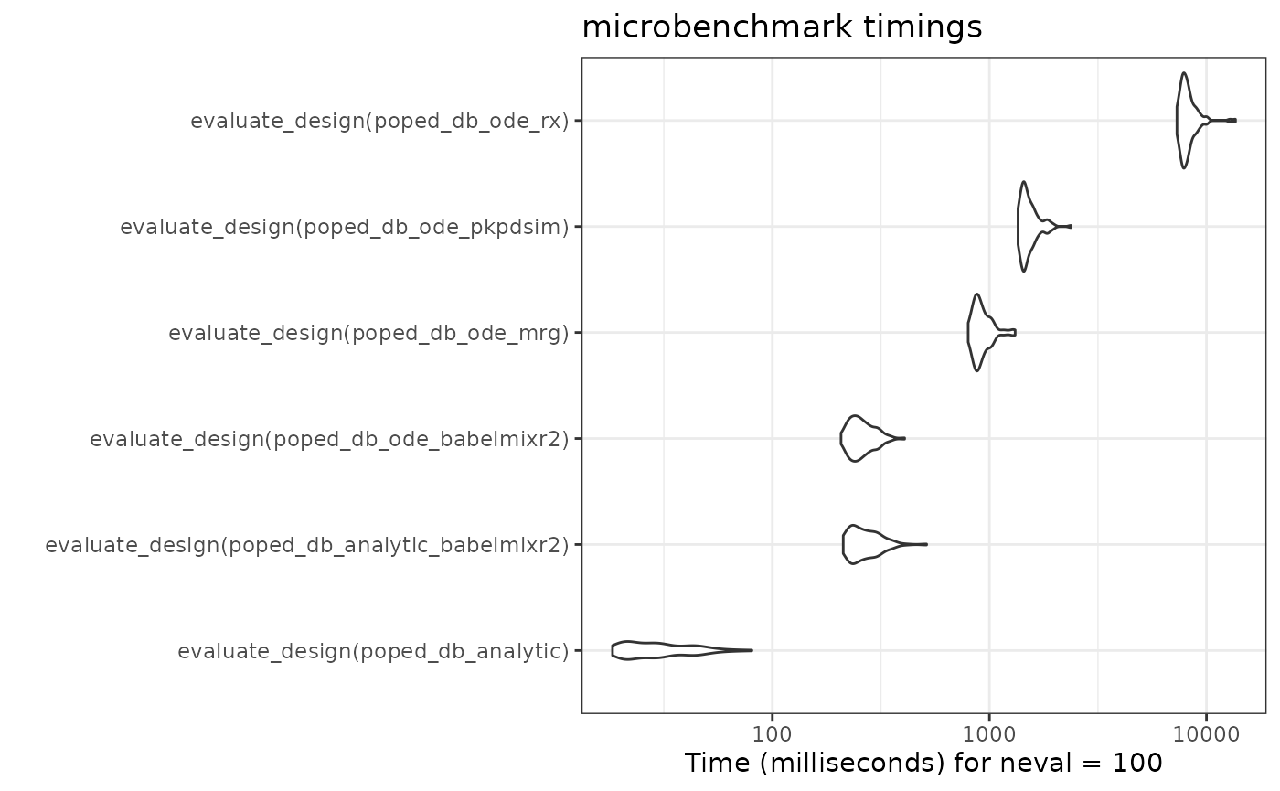

Note that the babelmixr2 ode solution is the fastest ode solver in this comparison. Among other things, this is because the model is loaded into memory and does not need to be setup each time. (As benchmarks, the mrgsolve, and PKPDsim implementations on the PopED’s website are included).

Also to me, the speed of all the tools are reasonable. In my opinion, the benefit of the babelmixr2 interface to PopED is the simplicity of using nlmixr2 / rxode2 functional models or fits directly in PopED without relying on conversions.

The interface is a bit different than the traditional PopED interface, and requires a design data-set as well as a popedControl() to setup a PopED database to run all of the PopED tasks. This is because traditionally nlmixr2 takes a dataset, “estimation” method and controls to change estimation method options.

babelmixr2 adopts the same paradigm of model, data, control to be applied to PopED. This should allow easy translation between the systems. With easier translation, hopefully optimal design in clinical trials will be easier to achieve.

Key notes to keep in mind

babelmixr2 loads models into memory and needs to keep track of which model is loaded. To help this you need to use babel.poped.database in place of create.poped.database when modifying babelmixr2 generated PopED databases. If this isn’t done, there is a chance that the model loaded will not be the expected loaded model and may either crash R or possibly give incorrect results.
babelmixr2 translates all error components to variances instead of the standard deviations in the nlmixr2/rxode2 model
When there are covariances in the omega specification, they will be identified as D[#,#] in the PopED output. To see what these numbers refer to it is helpful to see the name translations with $popedD.
Depending on your options, babelmixr2 may literally fix the model components, which means indexes may be different than you expect. The best way to get the correct index is use the babelmixr2 function babelBpopIdx() which is useful for using PopED
babelmixr2 uses model times in creating PopED databases; therefore models with modeling times in them cannot be used in this translation
babelmixr2 does not yet support inter-occasion variability models.

Where to find more examples

The examples from PopED have been converted to work with babelmixr2 and are available in the package and on GitHub

Matthew L. Fidler

Introduction – using babelmixr2 with PopED

babelmixr2 ODE solution

PopED/babelmixr2 event table description

Getting PopED functions from nlmixr2/rxode2 ui function

PopED’s ff_fun from babelmixr2

rxode2 models generated from babelmixr2

PopED’s fg_fun

PopED’s error function fError_fun

Other parameters generated by PopED

linear compartment models in babelmixr2