Create a Zero- and/or One-Inflated Beta Distribution
Beta01.RdClass and methods for zero- and/or one-inflated beta distributions in regression specification using the workflow from the distributions3 package.
Arguments
- mu
numeric. The mean of the beta distribution (on the open unit interval).
- phi
numeric. The precision parameter of the beta distribution.
- p0
numeric. The probability for an observation of zero (often referred to as zero inflation), by default set to
0.- p1
numeric. The probability for an observation of one (often referred to as one inflation), by default set to
0.
Details
The zero- and/or one-inflated beta distribution is obtained by adding point masses at zero and/or one to a standard beta distribution.
Note that the support of the standard beta distribution is the open unit interval where values of exactly zero or one cannot occur. Thus, the inflation jargon is rather misleading as there is no probability that could be inflated. It is rather a hurdle or two-part (or three-part) model.
Examples
#> Loading required namespace: distributions3
## package and random seed
library("distributions3")
#>
#> Attaching package: ‘distributions3’
#> The following object is masked from ‘package:stats’:
#>
#> Gamma
#> The following object is masked from ‘package:grDevices’:
#>
#> pdf
set.seed(6020)
## three beta distributions
X <- Beta01(
mu = c(0.25, 0.50, 0.75),
phi = c(1, 1, 2),
p0 = c(0.1, 0, 0),
p1 = c(0, 0, 0.3)
)
# \donttest{
X
#> [1] "Beta01(mu = 0.25, phi = 1, p0 = 0.1, p1 = 0.0)"
#> [2] "Beta01(mu = 0.50, phi = 1, p0 = 0.0, p1 = 0.0)"
#> [3] "Beta01(mu = 0.75, phi = 2, p0 = 0.0, p1 = 0.3)"
## compute moments of the distribution
mean(X)
#> [1] 0.225 0.500 0.825
variance(X)
#> [1] 0.090000 0.125000 0.056875
## support interval (minimum and maximum)
support(X)
#> min max
#> [1,] 0 1
#> [2,] 0 1
#> [3,] 0 1
## simulate random variables
random(X, 5)
#> r_1 r_2 r_3 r_4 r_5
#> [1,] 0.01770077 0.031967958 0.009185013 0.09774271 0.5297302
#> [2,] 0.11888790 0.004743561 0.209872794 0.56026234 0.7010201
#> [3,] 0.43181699 0.757365599 0.612582662 0.76991426 0.3122026
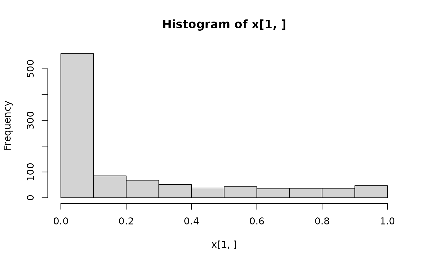
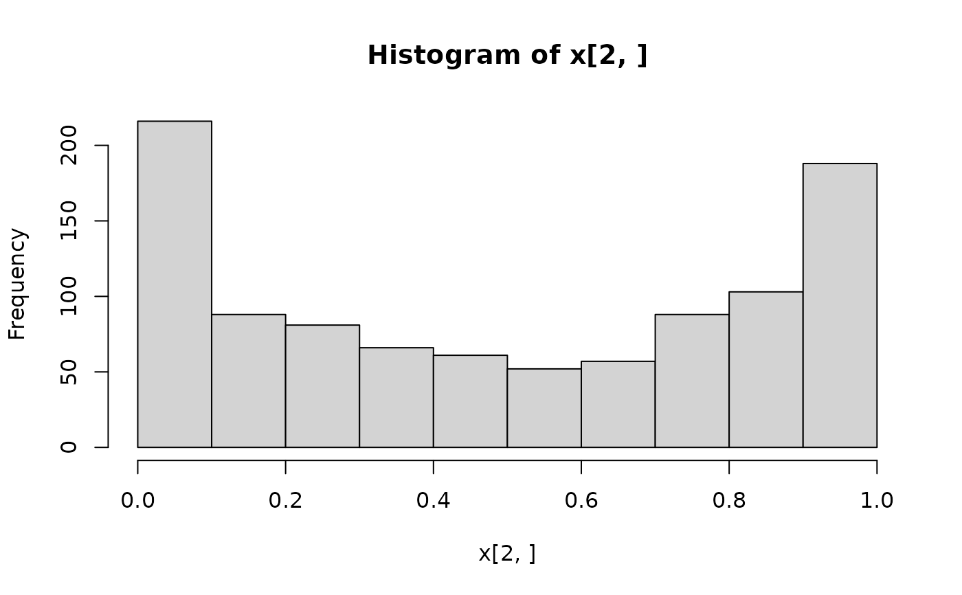
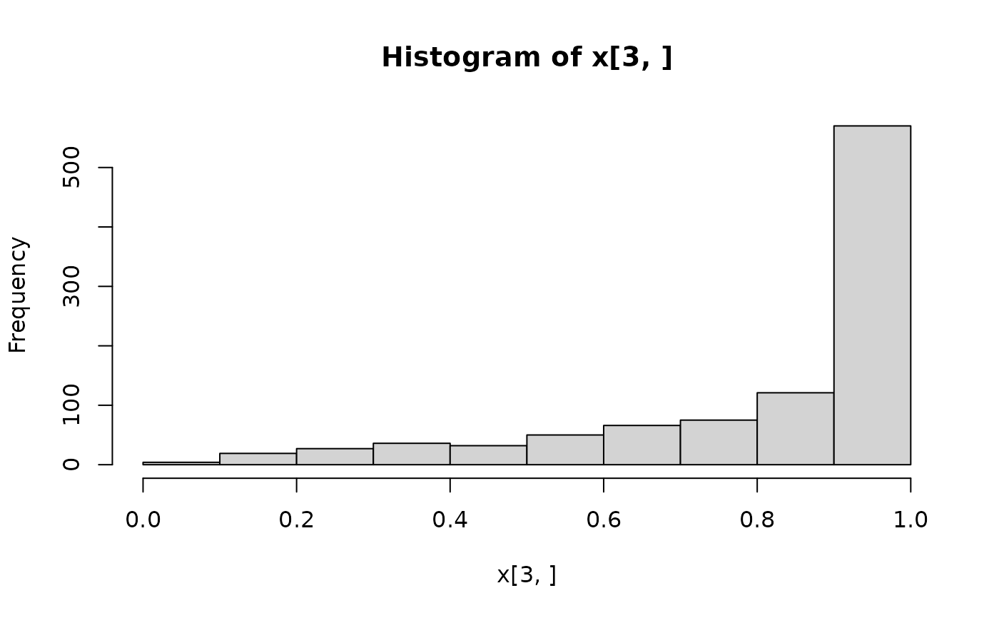
## histograms of 1,000 simulated observations
x <- random(X, 1000)
hist(x[1, ])
 hist(x[2, ])
 hist(x[3, ])
 ## probability density function (PDF) and log-density (or log-likelihood)
x <- c(0.25, 0.5, 0.75)
pdf(X, x)
#> [1] 0.6156832 0.6366198 0.7718605
pdf(X, x, log = TRUE)
#> [1] -0.4850227 -0.4515827 -0.2589515
log_pdf(X, x)
#> [1] -0.4850227 -0.4515827 -0.2589515
## cumulative distribution function (CDF)
cdf(X, x)
#> [1] 0.6808374 0.5000000 0.2737016
## quantiles
quantile(X, 0.5)
#> [1] 0.05868041 0.50000000 0.94876688
## cdf() and quantile() are inverses
cdf(X, quantile(X, 0.5))
#> [1] 0.5 0.5 0.5
quantile(X, cdf(X, 1))
#> [1] 1 1 1
## point mass probabilities (if any) on boundary
cdf(X, 0, lower.tail = TRUE)
#> [1] 0.1 0.0 0.0
cdf(X, 1, lower.tail = FALSE)
#> [1] 0.0 0.0 0.3
## all methods above can either be applied elementwise or for
## all combinations of X and x, if length(X) = length(x),
## also the result can be assured to be a matrix via drop = FALSE
p <- c(0.05, 0.5, 0.95)
quantile(X, p, elementwise = FALSE)
#> q_0.05 q_0.5 q_0.95
#> [1,] 0.00000000 0.05868041 0.8991438
#> [2,] 0.00615583 0.50000000 0.9938442
#> [3,] 0.28573175 0.94876688 1.0000000
quantile(X, p, elementwise = TRUE)
#> [1] 0.0 0.5 1.0
quantile(X, p, elementwise = TRUE, drop = FALSE)
#> quantile
#> [1,] 0.0
#> [2,] 0.5
#> [3,] 1.0
## compare theoretical and empirical mean from 1,000 simulated observations
cbind(
"theoretical" = mean(X),
"empirical" = rowMeans(random(X, 1000))
)
#> theoretical empirical
#> [1,] 0.225 0.2275291
#> [2,] 0.500 0.5091324
#> [3,] 0.825 0.8103725
# }
## probability density function (PDF) and log-density (or log-likelihood)
x <- c(0.25, 0.5, 0.75)
pdf(X, x)
#> [1] 0.6156832 0.6366198 0.7718605
pdf(X, x, log = TRUE)
#> [1] -0.4850227 -0.4515827 -0.2589515
log_pdf(X, x)
#> [1] -0.4850227 -0.4515827 -0.2589515
## cumulative distribution function (CDF)
cdf(X, x)
#> [1] 0.6808374 0.5000000 0.2737016
## quantiles
quantile(X, 0.5)
#> [1] 0.05868041 0.50000000 0.94876688
## cdf() and quantile() are inverses
cdf(X, quantile(X, 0.5))
#> [1] 0.5 0.5 0.5
quantile(X, cdf(X, 1))
#> [1] 1 1 1
## point mass probabilities (if any) on boundary
cdf(X, 0, lower.tail = TRUE)
#> [1] 0.1 0.0 0.0
cdf(X, 1, lower.tail = FALSE)
#> [1] 0.0 0.0 0.3
## all methods above can either be applied elementwise or for
## all combinations of X and x, if length(X) = length(x),
## also the result can be assured to be a matrix via drop = FALSE
p <- c(0.05, 0.5, 0.95)
quantile(X, p, elementwise = FALSE)
#> q_0.05 q_0.5 q_0.95
#> [1,] 0.00000000 0.05868041 0.8991438
#> [2,] 0.00615583 0.50000000 0.9938442
#> [3,] 0.28573175 0.94876688 1.0000000
quantile(X, p, elementwise = TRUE)
#> [1] 0.0 0.5 1.0
quantile(X, p, elementwise = TRUE, drop = FALSE)
#> quantile
#> [1,] 0.0
#> [2,] 0.5
#> [3,] 1.0
## compare theoretical and empirical mean from 1,000 simulated observations
cbind(
"theoretical" = mean(X),
"empirical" = rowMeans(random(X, 1000))
)
#> theoretical empirical
#> [1,] 0.225 0.2275291
#> [2,] 0.500 0.5091324
#> [3,] 0.825 0.8103725
# }