Create a 4-Parameter Beta Distribution

Class and methods for 4-parameter beta distributions in regression specification using the workflow from the distributions3 package.

Usage

Beta4(mu = numeric(), phi = numeric(), theta1 = NULL, theta2 = NULL)

Arguments

mu: numeric. The mean of the beta distribution that is extended to support [theta1, theta2].
phi: numeric. The precision parameter of the beta distribution that is extended to support [theta1, theta2].
theta1, theta2: numeric. The minimum and maximum, respectively, of the 4-parameter beta distribution. By default a symmetric support is chosen with theta1 set to 0 and theta2 = 1 - theta1 which thus corresponds to the classic beta distribution.

Details

The distribution is obtained by a linear transformation of a beta-distributed random variable with intercept theta1 and slope theta2 - theta1.

Value

A Beta4 distribution object.

Examples

## package and random seed
library("distributions3")
set.seed(6020)

## three beta distributions
X <- Beta4(
  mu  = c(0.25, 0.50, 0.75),
  phi = c(1, 1, 2),
  theta1 = c(0, -0.1, -0.1),
  theta2 = c(1, 1.1, 1.5)
)
# \donttest{
X
#> [1] "Beta4(mu = 0.25, phi = 1, theta1 =  0.0, theta2 = 1.0)"
#> [2] "Beta4(mu = 0.50, phi = 1, theta1 = -0.1, theta2 = 1.1)"
#> [3] "Beta4(mu = 0.75, phi = 2, theta1 = -0.1, theta2 = 1.5)"

## compute moments of the distribution
mean(X)
#> [1] 0.25 0.50 1.10
variance(X)
#> [1] 0.09375 0.18000 0.16000

## support interval (minimum and maximum)
support(X)
#>       min max
#> [1,]  0.0 1.0
#> [2,] -0.1 1.1
#> [3,] -0.1 1.5

## simulate random variables
random(X, 5)
#>            r_1       r_2         r_3        r_4         r_5
#> [1,] 0.7497152 0.8385523  0.03196796 0.91882879  0.54543668
#> [2,] 0.1263742 1.0978772 -0.09430773 0.07151503 -0.00499443
#> [3,] 1.4311350 1.4850582  1.11178496 1.36985916  1.24450679

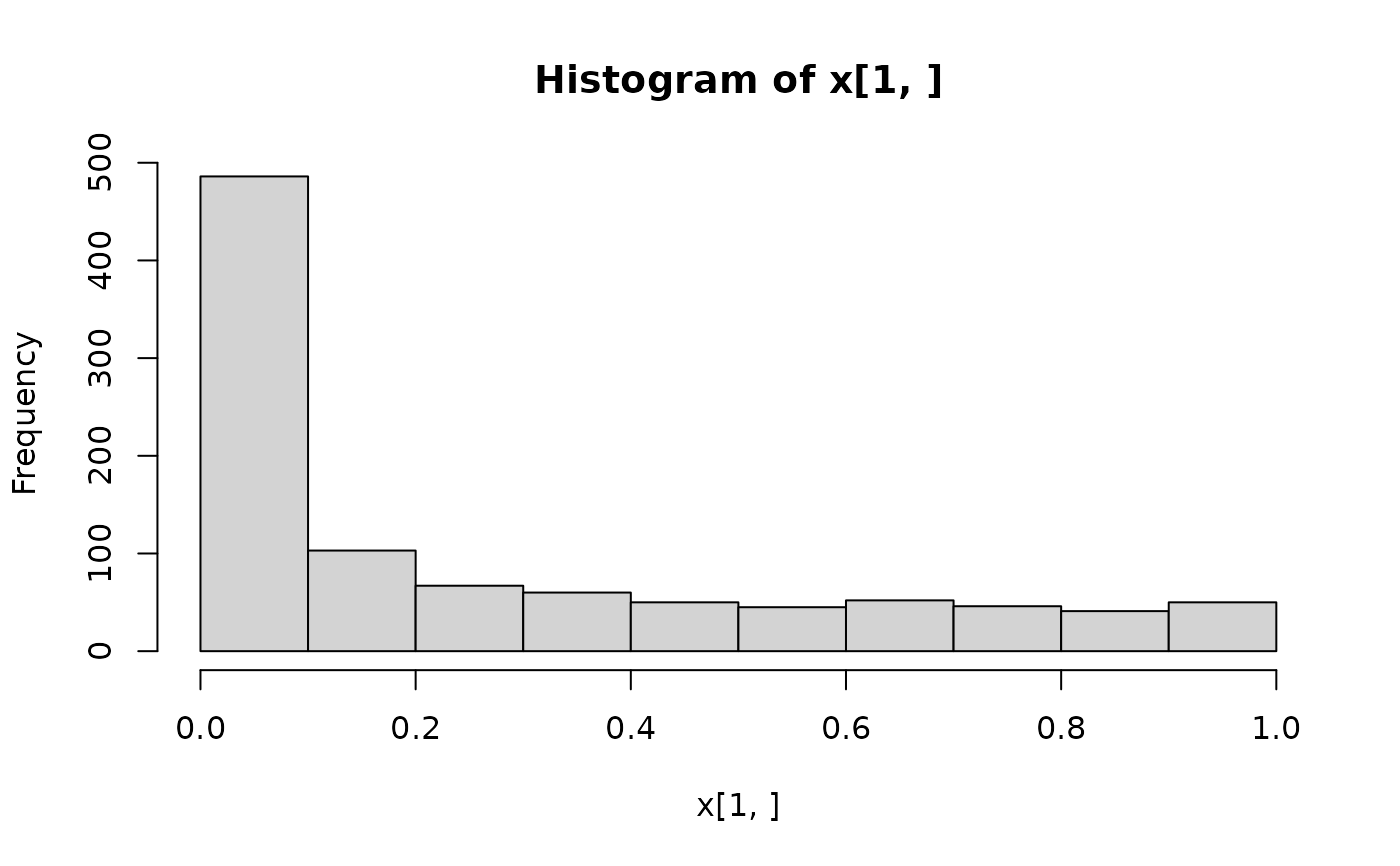
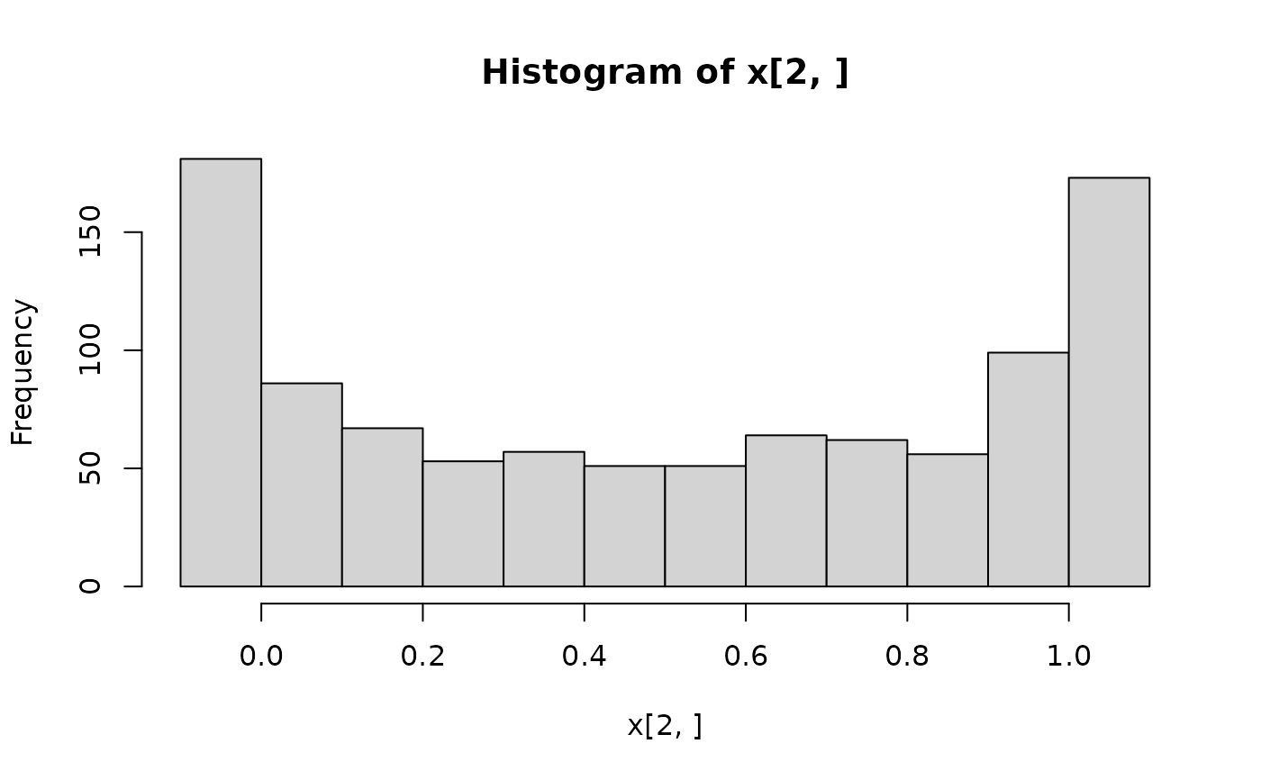
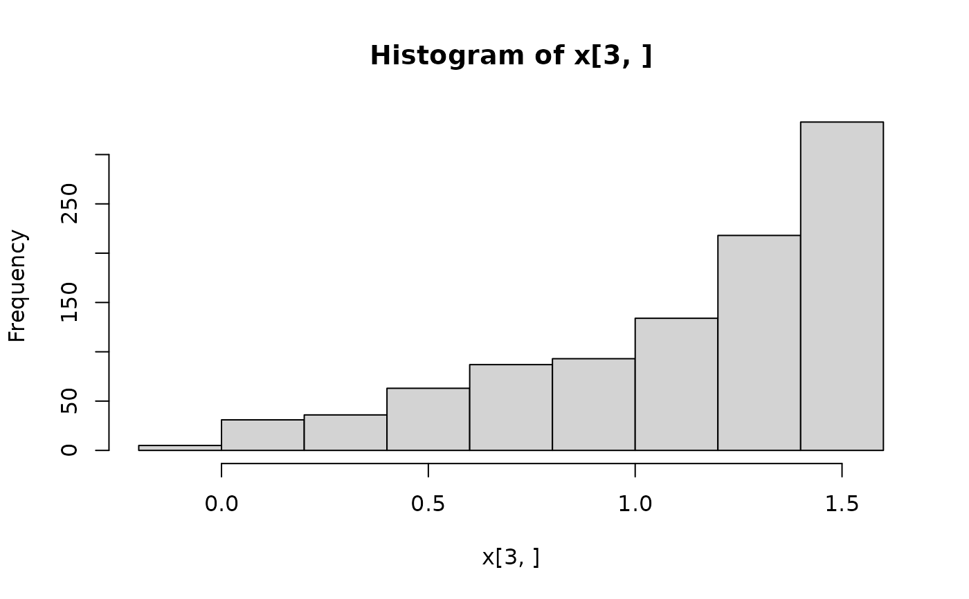
## histograms of 1,000 simulated observations
x <- random(X, 1000)
hist(x[1, ])

hist(x[2, ])

hist(x[3, ])


## probability density function (PDF) and log-density (or log-likelihood)
x <- c(0.25, 0.5, 0.75)
pdf(X, x)
#> [1] 0.6840925 0.5305165 0.4235834
pdf(X, x, log = TRUE)
#> [1] -0.3796622 -0.6339043 -0.8590048
log_pdf(X, x)
#> [1] -0.3796622 -0.6339043 -0.8590048

## cumulative distribution function (CDF)
cdf(X, x)
#> [1] 0.6453748 0.5000000 0.2022198

## quantiles
quantile(X, 0.5)
#> [1] 0.09331223 0.50000000 1.23888962

## cdf() and quantile() are inverses
cdf(X, quantile(X, 0.5))
#> [1] 0.5 0.5 0.5
quantile(X, cdf(X, 1))
#> [1] 1 1 1

## all methods above can either be applied elementwise or for
## all combinations of X and x, if length(X) = length(x),
## also the result can be assured to be a matrix via drop = FALSE
p <- c(0.05, 0.5, 0.95)
quantile(X, p, elementwise = FALSE)
#>             q_0.05      q_0.5    q_0.95
#> [1,]  9.512588e-06 0.09331223 0.9118445
#> [2,] -9.261300e-02 0.50000000 1.0926130
#> [3,]  2.656317e-01 1.23888962 1.4975313
quantile(X, p, elementwise = TRUE)
#> [1] 9.512588e-06 5.000000e-01 1.497531e+00
quantile(X, p, elementwise = TRUE, drop = FALSE)
#>          quantile
#> [1,] 9.512588e-06
#> [2,] 5.000000e-01
#> [3,] 1.497531e+00

## compare theoretical and empirical mean from 1,000 simulated observations
cbind(
  "theoretical" = mean(X),
  "empirical" = rowMeans(random(X, 1000))
)
#>      theoretical empirical
#> [1,]        0.25 0.2464581
#> [2,]        0.50 0.4930360
#> [3,]        1.10 1.1068752
# }