Tidy summarizes information about the components of a model. A model component might be a single term in a regression, a single hypothesis, a cluster, or a class. Exactly what tidy considers to be a model component varies across models but is usually self-evident. If a model has several distinct types of components, you will need to specify which components to return.
# S3 method for class 'gmm'
tidy(x, conf.int = FALSE, conf.level = 0.95, exponentiate = FALSE, ...)
Arguments
- x
A
gmmobject returned fromgmm::gmm().- conf.int
Logical indicating whether or not to include a confidence interval in the tidied output. Defaults to
FALSE.- conf.level
The confidence level to use for the confidence interval if
conf.int = TRUE. Must be strictly greater than 0 and less than 1. Defaults to 0.95, which corresponds to a 95 percent confidence interval.- exponentiate
Logical indicating whether or not to exponentiate the the coefficient estimates. This is typical for logistic and multinomial regressions, but a bad idea if there is no log or logit link. Defaults to
FALSE.- ...
Additional arguments. Not used. Needed to match generic signature only. Cautionary note: Misspelled arguments will be absorbed in
..., where they will be ignored. If the misspelled argument has a default value, the default value will be used. For example, if you passconf.lvel = 0.9, all computation will proceed usingconf.level = 0.95. Two exceptions here are:
See also
Other gmm tidiers:
glance.gmm()
Value
A tibble::tibble() with columns:
- conf.high
Upper bound on the confidence interval for the estimate.
- conf.low
Lower bound on the confidence interval for the estimate.
- estimate
The estimated value of the regression term.
- p.value
The two-sided p-value associated with the observed statistic.
- statistic
The value of a T-statistic to use in a hypothesis that the regression term is non-zero.
- std.error
The standard error of the regression term.
- term
The name of the regression term.
Examples
# load libraries for models and data
library(gmm)
# examples come from the "gmm" package
# CAPM test with GMM
data(Finance)
r <- Finance[1:300, 1:10]
rm <- Finance[1:300, "rm"]
rf <- Finance[1:300, "rf"]
z <- as.matrix(r - rf)
t <- nrow(z)
zm <- rm - rf
h <- matrix(zm, t, 1)
res <- gmm(z ~ zm, x = h)
# tidy result
tidy(res)
#> # A tibble: 20 × 5
#> term estimate std.error statistic p.value
#> <chr> <dbl> <dbl> <dbl> <dbl>
#> 1 WMK_(Intercept) -0.00471 0.141 -0.0333 9.73e- 1
#> 2 UIS_(Intercept) 0.102 0.146 0.700 4.84e- 1
#> 3 ORB_(Intercept) 0.146 0.207 0.706 4.80e- 1
#> 4 MAT_(Intercept) 0.0359 0.138 0.260 7.95e- 1
#> 5 ABAX_(Intercept) 0.0917 0.282 0.325 7.45e- 1
#> 6 T_(Intercept) 0.0231 0.0770 0.300 7.64e- 1
#> 7 EMR_(Intercept) 0.0299 0.0559 0.535 5.93e- 1
#> 8 JCS_(Intercept) 0.117 0.152 0.766 4.44e- 1
#> 9 VOXX_(Intercept) 0.0209 0.206 0.101 9.19e- 1
#> 10 ZOOM_(Intercept) -0.219 0.208 -1.05 2.92e- 1
#> 11 WMK_zm 0.320 0.120 2.66 7.84e- 3
#> 12 UIS_zm 1.26 0.231 5.46 4.72e- 8
#> 13 ORB_zm 1.49 0.517 2.88 3.97e- 3
#> 14 MAT_zm 1.01 0.215 4.71 2.51e- 6
#> 15 ABAX_zm 1.09 0.580 1.88 6.03e- 2
#> 16 T_zm 0.849 0.196 4.34 1.45e- 5
#> 17 EMR_zm 0.745 0.105 7.07 1.53e-12
#> 18 JCS_zm 0.959 0.358 2.68 7.40e- 3
#> 19 VOXX_zm 1.48 0.378 3.92 8.73e- 5
#> 20 ZOOM_zm 2.08 0.307 6.76 1.35e-11
tidy(res, conf.int = TRUE)
#> # A tibble: 20 × 7
#> term estimate std.error statistic p.value conf.low conf.high
#> <chr> <dbl> <dbl> <dbl> <dbl> <dbl> <dbl>
#> 1 WMK_(Intercept) -0.00471 0.141 -0.0333 9.73e- 1 -0.282 0.272
#> 2 UIS_(Intercept) 0.102 0.146 0.700 4.84e- 1 -0.184 0.389
#> 3 ORB_(Intercept) 0.146 0.207 0.706 4.80e- 1 -0.259 0.551
#> 4 MAT_(Intercept) 0.0359 0.138 0.260 7.95e- 1 -0.235 0.307
#> 5 ABAX_(Intercept) 0.0917 0.282 0.325 7.45e- 1 -0.462 0.645
#> 6 T_(Intercept) 0.0231 0.0770 0.300 7.64e- 1 -0.128 0.174
#> 7 EMR_(Intercept) 0.0299 0.0559 0.535 5.93e- 1 -0.0796 0.139
#> 8 JCS_(Intercept) 0.117 0.152 0.766 4.44e- 1 -0.182 0.416
#> 9 VOXX_(Intercept) 0.0209 0.206 0.101 9.19e- 1 -0.383 0.425
#> 10 ZOOM_(Intercept) -0.219 0.208 -1.05 2.92e- 1 -0.626 0.188
#> 11 WMK_zm 0.320 0.120 2.66 7.84e- 3 0.0841 0.556
#> 12 UIS_zm 1.26 0.231 5.46 4.72e- 8 0.807 1.71
#> 13 ORB_zm 1.49 0.517 2.88 3.97e- 3 0.476 2.50
#> 14 MAT_zm 1.01 0.215 4.71 2.51e- 6 0.591 1.43
#> 15 ABAX_zm 1.09 0.580 1.88 6.03e- 2 -0.0472 2.23
#> 16 T_zm 0.849 0.196 4.34 1.45e- 5 0.465 1.23
#> 17 EMR_zm 0.745 0.105 7.07 1.53e-12 0.538 0.951
#> 18 JCS_zm 0.959 0.358 2.68 7.40e- 3 0.257 1.66
#> 19 VOXX_zm 1.48 0.378 3.92 8.73e- 5 0.742 2.22
#> 20 ZOOM_zm 2.08 0.307 6.76 1.35e-11 1.48 2.68
tidy(res, conf.int = TRUE, conf.level = .99)
#> # A tibble: 20 × 7
#> term estimate std.error statistic p.value conf.low conf.high
#> <chr> <dbl> <dbl> <dbl> <dbl> <dbl> <dbl>
#> 1 WMK_(Intercept) -0.00471 0.141 -0.0333 9.73e- 1 -0.369 0.359
#> 2 UIS_(Intercept) 0.102 0.146 0.700 4.84e- 1 -0.274 0.479
#> 3 ORB_(Intercept) 0.146 0.207 0.706 4.80e- 1 -0.387 0.679
#> 4 MAT_(Intercept) 0.0359 0.138 0.260 7.95e- 1 -0.320 0.392
#> 5 ABAX_(Intercept) 0.0917 0.282 0.325 7.45e- 1 -0.636 0.819
#> 6 T_(Intercept) 0.0231 0.0770 0.300 7.64e- 1 -0.175 0.222
#> 7 EMR_(Intercept) 0.0299 0.0559 0.535 5.93e- 1 -0.114 0.174
#> 8 JCS_(Intercept) 0.117 0.152 0.766 4.44e- 1 -0.276 0.510
#> 9 VOXX_(Intercept) 0.0209 0.206 0.101 9.19e- 1 -0.510 0.552
#> 10 ZOOM_(Intercept) -0.219 0.208 -1.05 2.92e- 1 -0.754 0.316
#> 11 WMK_zm 0.320 0.120 2.66 7.84e- 3 0.0100 0.630
#> 12 UIS_zm 1.26 0.231 5.46 4.72e- 8 0.665 1.85
#> 13 ORB_zm 1.49 0.517 2.88 3.97e- 3 0.157 2.82
#> 14 MAT_zm 1.01 0.215 4.71 2.51e- 6 0.458 1.57
#> 15 ABAX_zm 1.09 0.580 1.88 6.03e- 2 -0.404 2.58
#> 16 T_zm 0.849 0.196 4.34 1.45e- 5 0.345 1.35
#> 17 EMR_zm 0.745 0.105 7.07 1.53e-12 0.473 1.02
#> 18 JCS_zm 0.959 0.358 2.68 7.40e- 3 0.0367 1.88
#> 19 VOXX_zm 1.48 0.378 3.92 8.73e- 5 0.509 2.46
#> 20 ZOOM_zm 2.08 0.307 6.76 1.35e-11 1.29 2.87
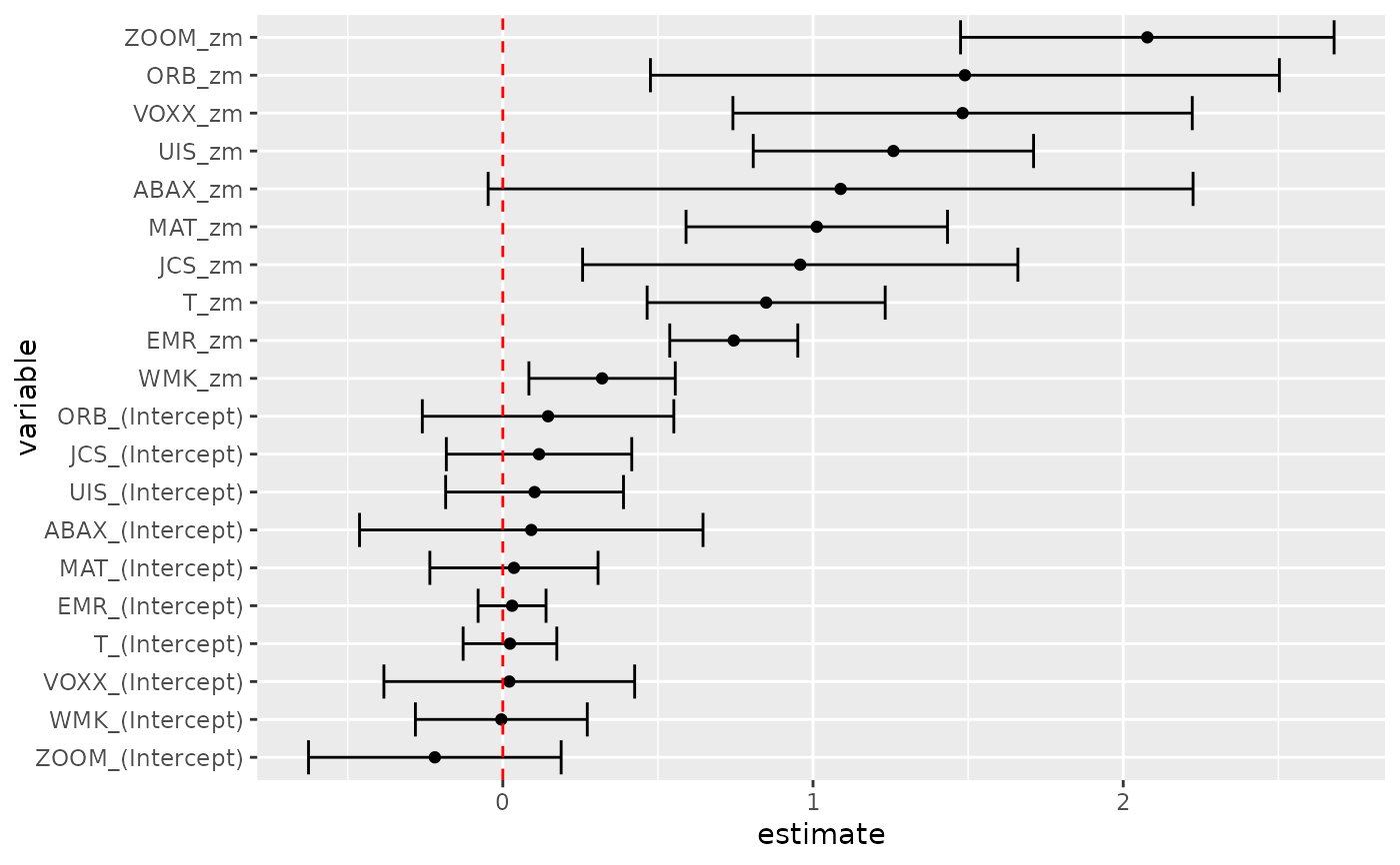
# coefficient plot
library(ggplot2)
library(dplyr)
tidy(res, conf.int = TRUE) %>%
mutate(variable = reorder(term, estimate)) %>%
ggplot(aes(estimate, variable)) +
geom_point() +
geom_errorbarh(aes(xmin = conf.low, xmax = conf.high)) +
geom_vline(xintercept = 0, color = "red", lty = 2)
 # from a function instead of a matrix
g <- function(theta, x) {
e <- x[, 2:11] - theta[1] - (x[, 1] - theta[1]) %*% matrix(theta[2:11], 1, 10)
gmat <- cbind(e, e * c(x[, 1]))
return(gmat)
}
x <- as.matrix(cbind(rm, r))
res_black <- gmm(g, x = x, t0 = rep(0, 11))
#> Warning: model order: 1 singularities in the computation of the projection matrix results are only valid up to model order 0
#> Error in AA %*% t(X) : requires numeric/complex matrix/vector arguments
#> Error in AllArg$bw(obj, order.by = AllArg$order.by, kernel = AllArg$kernel, prewhite = AllArg$prewhite, ar.method = AllArg$ar.method, approx = AllArg$approx): VAR(1) prewhitening of estimating functions failed
tidy(res_black)
#> Error: object 'res_black' not found
tidy(res_black, conf.int = TRUE)
#> Error: object 'res_black' not found
# APT test with Fama-French factors and GMM
f1 <- zm
f2 <- Finance[1:300, "hml"] - rf
f3 <- Finance[1:300, "smb"] - rf
h <- cbind(f1, f2, f3)
res2 <- gmm(z ~ f1 + f2 + f3, x = h)
td2 <- tidy(res2, conf.int = TRUE)
td2
#> # A tibble: 40 × 7
#> term estimate std.error statistic p.value conf.low conf.high
#> <chr> <dbl> <dbl> <dbl> <dbl> <dbl> <dbl>
#> 1 WMK_(Intercept) -0.0127 0.146 -0.0873 0.930 -0.299 0.273
#> 2 UIS_(Intercept) 0.0799 0.311 0.257 0.797 -0.529 0.689
#> 3 ORB_(Intercept) 0.135 0.263 0.514 0.608 -0.381 0.652
#> 4 MAT_(Intercept) 0.0405 0.321 0.126 0.900 -0.589 0.670
#> 5 ABAX_(Intercept) 0.0589 0.584 0.101 0.920 -1.09 1.20
#> 6 T_(Intercept) 0.0337 0.316 0.107 0.915 -0.586 0.653
#> 7 EMR_(Intercept) 0.0304 0.180 0.169 0.866 -0.323 0.383
#> 8 JCS_(Intercept) 0.0994 0.403 0.247 0.805 -0.690 0.889
#> 9 VOXX_(Intercept) -0.0108 0.389 -0.0279 0.978 -0.774 0.752
#> 10 ZOOM_(Intercept) -0.163 0.531 -0.306 0.759 -1.20 0.878
#> # ℹ 30 more rows
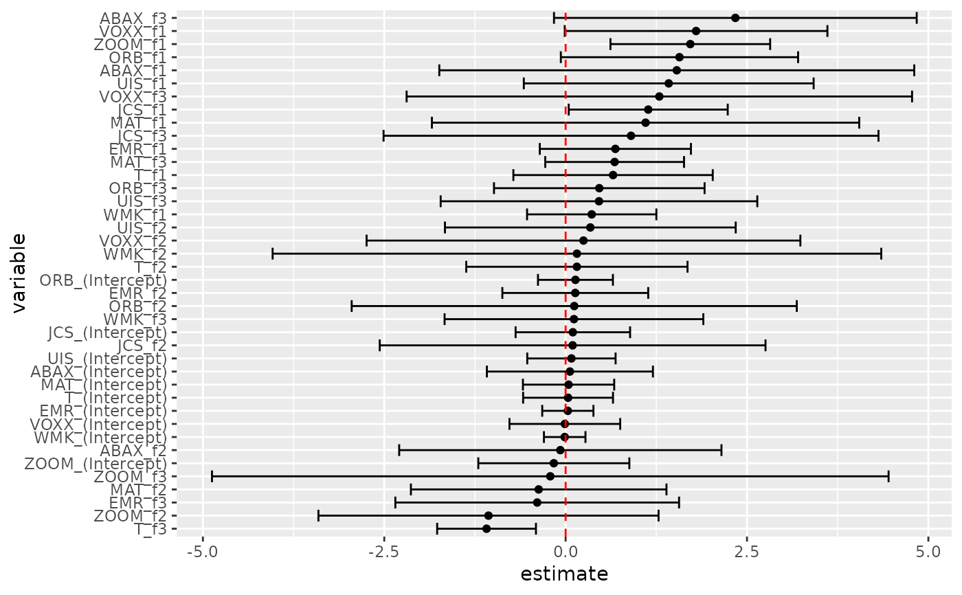
# coefficient plot
td2 %>%
mutate(variable = reorder(term, estimate)) %>%
ggplot(aes(estimate, variable)) +
geom_point() +
geom_errorbarh(aes(xmin = conf.low, xmax = conf.high)) +
geom_vline(xintercept = 0, color = "red", lty = 2)
# from a function instead of a matrix
g <- function(theta, x) {
e <- x[, 2:11] - theta[1] - (x[, 1] - theta[1]) %*% matrix(theta[2:11], 1, 10)
gmat <- cbind(e, e * c(x[, 1]))
return(gmat)
}
x <- as.matrix(cbind(rm, r))
res_black <- gmm(g, x = x, t0 = rep(0, 11))
#> Warning: model order: 1 singularities in the computation of the projection matrix results are only valid up to model order 0
#> Error in AA %*% t(X) : requires numeric/complex matrix/vector arguments
#> Error in AllArg$bw(obj, order.by = AllArg$order.by, kernel = AllArg$kernel, prewhite = AllArg$prewhite, ar.method = AllArg$ar.method, approx = AllArg$approx): VAR(1) prewhitening of estimating functions failed
tidy(res_black)
#> Error: object 'res_black' not found
tidy(res_black, conf.int = TRUE)
#> Error: object 'res_black' not found
# APT test with Fama-French factors and GMM
f1 <- zm
f2 <- Finance[1:300, "hml"] - rf
f3 <- Finance[1:300, "smb"] - rf
h <- cbind(f1, f2, f3)
res2 <- gmm(z ~ f1 + f2 + f3, x = h)
td2 <- tidy(res2, conf.int = TRUE)
td2
#> # A tibble: 40 × 7
#> term estimate std.error statistic p.value conf.low conf.high
#> <chr> <dbl> <dbl> <dbl> <dbl> <dbl> <dbl>
#> 1 WMK_(Intercept) -0.0127 0.146 -0.0873 0.930 -0.299 0.273
#> 2 UIS_(Intercept) 0.0799 0.311 0.257 0.797 -0.529 0.689
#> 3 ORB_(Intercept) 0.135 0.263 0.514 0.608 -0.381 0.652
#> 4 MAT_(Intercept) 0.0405 0.321 0.126 0.900 -0.589 0.670
#> 5 ABAX_(Intercept) 0.0589 0.584 0.101 0.920 -1.09 1.20
#> 6 T_(Intercept) 0.0337 0.316 0.107 0.915 -0.586 0.653
#> 7 EMR_(Intercept) 0.0304 0.180 0.169 0.866 -0.323 0.383
#> 8 JCS_(Intercept) 0.0994 0.403 0.247 0.805 -0.690 0.889
#> 9 VOXX_(Intercept) -0.0108 0.389 -0.0279 0.978 -0.774 0.752
#> 10 ZOOM_(Intercept) -0.163 0.531 -0.306 0.759 -1.20 0.878
#> # ℹ 30 more rows
# coefficient plot
td2 %>%
mutate(variable = reorder(term, estimate)) %>%
ggplot(aes(estimate, variable)) +
geom_point() +
geom_errorbarh(aes(xmin = conf.low, xmax = conf.high)) +
geom_vline(xintercept = 0, color = "red", lty = 2)