Tidy summarizes information about the components of a model. A model component might be a single term in a regression, a single hypothesis, a cluster, or a class. Exactly what tidy considers to be a model component varies across models but is usually self-evident. If a model has several distinct types of components, you will need to specify which components to return.
# S3 method for class 'survfit'
tidy(x, ...)
Arguments
- x
An
survfitobject returned fromsurvival::survfit().- ...
For
glance.survfit(), additional arguments passed tosummary(). Otherwise ignored.
See also
Other survival tidiers:
augment.coxph(),
augment.survreg(),
glance.aareg(),
glance.cch(),
glance.coxph(),
glance.pyears(),
glance.survdiff(),
glance.survexp(),
glance.survfit(),
glance.survreg(),
tidy.aareg(),
tidy.cch(),
tidy.coxph(),
tidy.pyears(),
tidy.survdiff(),
tidy.survexp(),
tidy.survreg()
Value
A tibble::tibble() with columns:
- conf.high
Upper bound on the confidence interval for the estimate.
- conf.low
Lower bound on the confidence interval for the estimate.
- n.censor
Number of censored events.
- n.event
Number of events at time t.
- n.risk
Number of individuals at risk at time zero.
- std.error
The standard error of the regression term.
- time
Point in time.
- estimate
estimate of survival or cumulative incidence rate when multistate
- state
state if multistate survfit object input
- strata
strata if stratified survfit object input
Examples
# load libraries for models and data
library(survival)
# fit model
cfit <- coxph(Surv(time, status) ~ age + sex, lung)
sfit <- survfit(cfit)
# summarize model fit with tidiers + visualization
tidy(sfit)
#> # A tibble: 186 × 8
#> time n.risk n.event n.censor estimate std.error conf.high conf.low
#> <dbl> <dbl> <dbl> <dbl> <dbl> <dbl> <dbl> <dbl>
#> 1 5 228 1 0 0.996 0.00419 1 0.988
#> 2 11 227 3 0 0.983 0.00845 1.00 0.967
#> 3 12 224 1 0 0.979 0.00947 0.997 0.961
#> 4 13 223 2 0 0.971 0.0113 0.992 0.949
#> 5 15 221 1 0 0.966 0.0121 0.990 0.944
#> 6 26 220 1 0 0.962 0.0129 0.987 0.938
#> 7 30 219 1 0 0.958 0.0136 0.984 0.933
#> 8 31 218 1 0 0.954 0.0143 0.981 0.927
#> 9 53 217 2 0 0.945 0.0157 0.975 0.917
#> 10 54 215 1 0 0.941 0.0163 0.972 0.911
#> # ℹ 176 more rows
glance(sfit)
#> # A tibble: 1 × 10
#> records n.max n.start events rmean rmean.std.error median conf.low conf.high
#> <dbl> <dbl> <dbl> <dbl> <dbl> <dbl> <dbl> <dbl> <dbl>
#> 1 228 228 228 165 381. 20.3 320 285 363
#> # ℹ 1 more variable: nobs <int>
library(ggplot2)
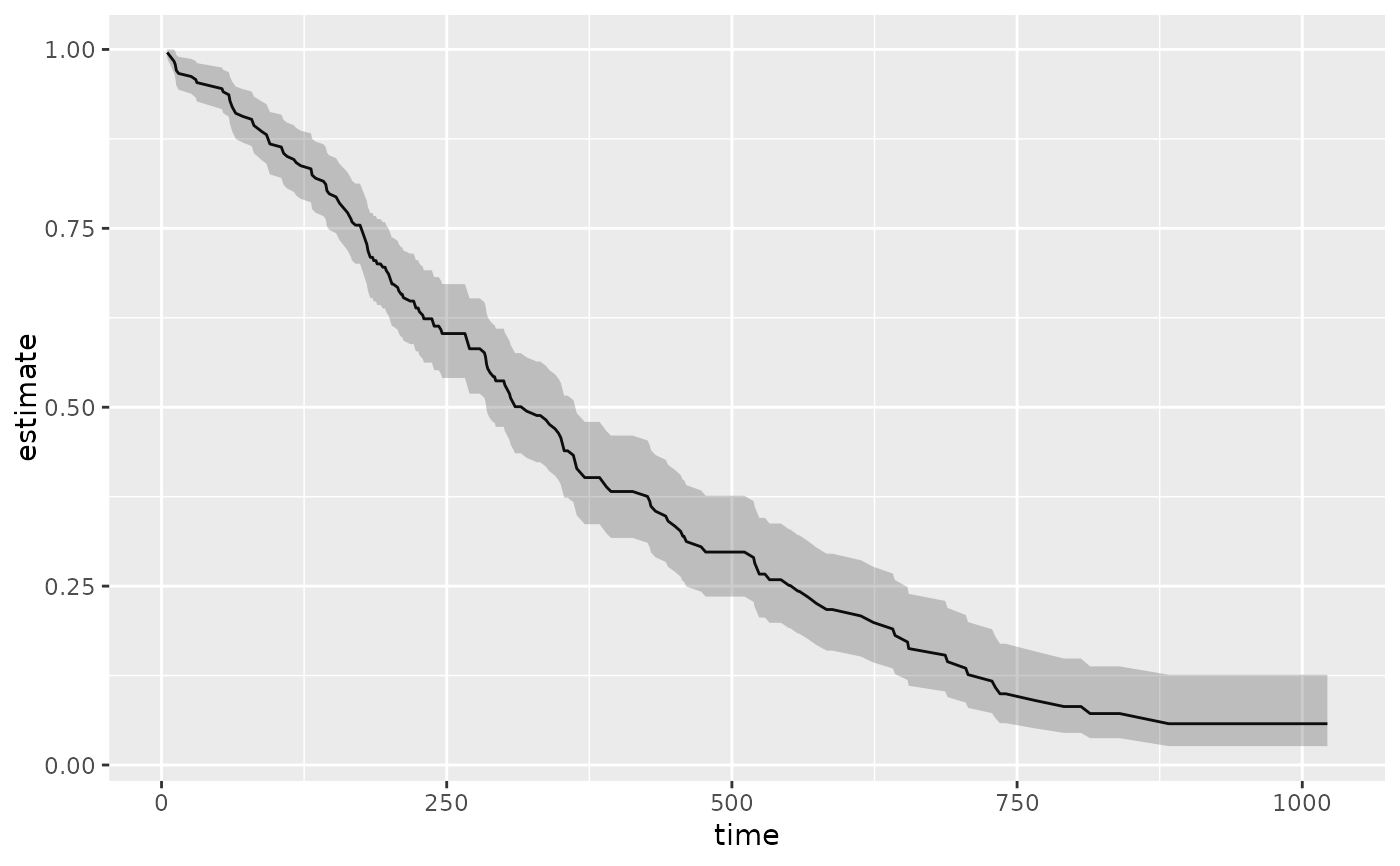
ggplot(tidy(sfit), aes(time, estimate)) +
geom_line() +
geom_ribbon(aes(ymin = conf.low, ymax = conf.high), alpha = .25)
 # multi-state
fitCI <- survfit(Surv(stop, status * as.numeric(event), type = "mstate") ~ 1,
data = mgus1, subset = (start == 0)
)
td_multi <- tidy(fitCI)
td_multi
#> # A tibble: 711 × 9
#> time n.risk n.event n.censor estimate std.error conf.high conf.low state
#> <dbl> <dbl> <dbl> <dbl> <dbl> <dbl> <dbl> <dbl> <chr>
#> 1 6 241 0 0 0.996 0.00414 1 0.988 (s0)
#> 2 7 240 0 0 0.992 0.00584 1 0.980 (s0)
#> 3 31 239 0 0 0.988 0.00714 1 0.974 (s0)
#> 4 32 238 0 0 0.983 0.00823 1.00 0.967 (s0)
#> 5 39 237 0 0 0.979 0.00918 0.997 0.961 (s0)
#> 6 60 236 0 0 0.975 0.0100 0.995 0.956 (s0)
#> 7 61 235 0 0 0.967 0.0115 0.990 0.944 (s0)
#> 8 152 233 0 0 0.963 0.0122 0.987 0.939 (s0)
#> 9 153 232 0 0 0.959 0.0128 0.984 0.934 (s0)
#> 10 174 231 0 0 0.954 0.0134 0.981 0.928 (s0)
#> # ℹ 701 more rows
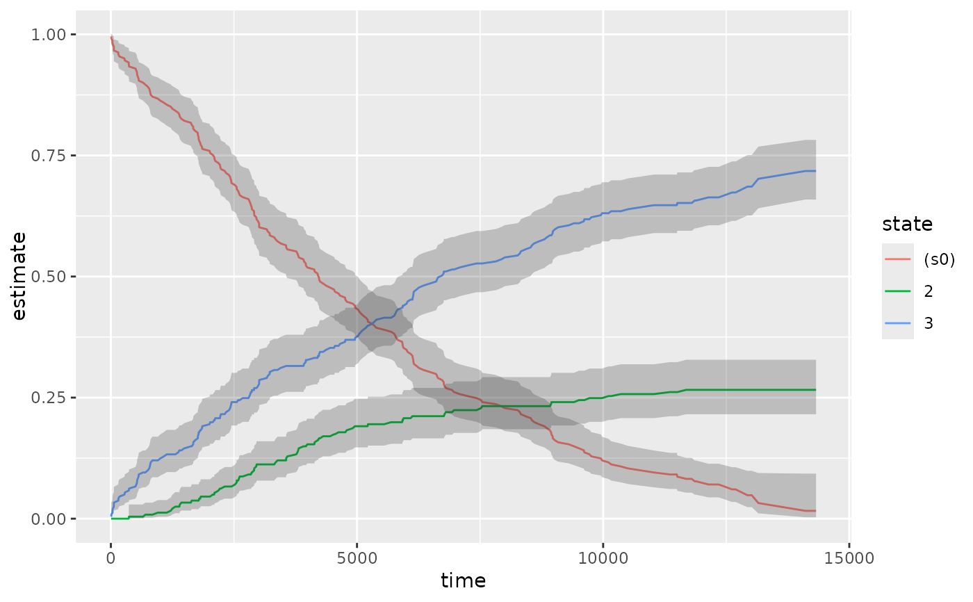
ggplot(td_multi, aes(time, estimate, group = state)) +
geom_line(aes(color = state)) +
geom_ribbon(aes(ymin = conf.low, ymax = conf.high), alpha = .25)
# multi-state
fitCI <- survfit(Surv(stop, status * as.numeric(event), type = "mstate") ~ 1,
data = mgus1, subset = (start == 0)
)
td_multi <- tidy(fitCI)
td_multi
#> # A tibble: 711 × 9
#> time n.risk n.event n.censor estimate std.error conf.high conf.low state
#> <dbl> <dbl> <dbl> <dbl> <dbl> <dbl> <dbl> <dbl> <chr>
#> 1 6 241 0 0 0.996 0.00414 1 0.988 (s0)
#> 2 7 240 0 0 0.992 0.00584 1 0.980 (s0)
#> 3 31 239 0 0 0.988 0.00714 1 0.974 (s0)
#> 4 32 238 0 0 0.983 0.00823 1.00 0.967 (s0)
#> 5 39 237 0 0 0.979 0.00918 0.997 0.961 (s0)
#> 6 60 236 0 0 0.975 0.0100 0.995 0.956 (s0)
#> 7 61 235 0 0 0.967 0.0115 0.990 0.944 (s0)
#> 8 152 233 0 0 0.963 0.0122 0.987 0.939 (s0)
#> 9 153 232 0 0 0.959 0.0128 0.984 0.934 (s0)
#> 10 174 231 0 0 0.954 0.0134 0.981 0.928 (s0)
#> # ℹ 701 more rows
ggplot(td_multi, aes(time, estimate, group = state)) +
geom_line(aes(color = state)) +
geom_ribbon(aes(ymin = conf.low, ymax = conf.high), alpha = .25)