Plot Categorical Regression Spline Fits

Plot fitted conditional mean, conditional quantile, gradient, and bivariate surface displays for crs objects using the modern np-style plot interface. This page is the canonical reference for CRS plot options and plot control helper objects.

Usage

# S3 method for class 'crs'
plot(x, ...)

crs_boot_control(wild = c("rademacher", "mammen"),
                 blocklen = NULL,
                 ...)

crs_grid_control(xtrim = NULL, xq = NULL, slices = NULL)

Arguments

Plot Object

This argument identifies the fitted CRS object to plot.

x: an object of class "crs" returned by crs. Mean-regression objects plot fitted conditional means by default. Objects fit with tau plot fitted conditional quantiles.

Control Helper Constructors

These arguments configure optional S3 control objects consumed by CRS plot methods. The crs_*_control() helpers use the same argument conventions as the corresponding modern np plot controls where the CRS plot route supports the same feature.

wild: wild-bootstrap multiplier family.
blocklen: optional positive block length for bootstrap="fixed" and bootstrap="geom". If omitted for mean crs plots, CRS uses the same automatic block-length selector as np.
xtrim: optional scalar trimming/expansion control stored on a grid control object. This uses the same scalar CRS contract as the top-level xtrim argument documented below.
xq: optional conditioning quantile or vector of conditioning quantiles.
slices: reserved for future explicit slice selection.

Plot Options Passed Through `...`

Named options passed via ... include:

Data and evaluation controls

grid_control: optional detailed grid controls created by crs_grid_control.
neval: the number of evaluation points used for each plotted continuous margin. For bivariate surfaces, the plotted grid has neval * neval evaluation points.
xq: the conditioning quantile used to hold non-plotted continuous variables fixed when drawing one-dimensional slices.
xtrim: scalar trimming/expansion control for the evaluation support. Values in [0,0.5) trim both tails by the requested quantile amount; negative values expand the support. The default evaluates over the observed support of the plotted continuous variable.

Plot content controls

common_scale: logical; whether multiple one-dimensional panels should share a common vertical scale when feasible.
gradient_order, gradients: derivative plotting controls. gradients=TRUE requests gradients/effects rather than the fitted function, and gradient_order selects the derivative order. Current CRS gradient plotting requires a scalar gradient_order.
layout: "auto" or TRUE requests automatic par(mfrow=...) management for multi-panel plots. "current" or FALSE preserves the user's current graphics layout.
output: one of "plot", "data", or "both". "both" is the public spelling for the historical "plot-data" behavior. "data" returns the plotting payload without drawing.

Interval and bootstrap controls

alpha: the nominal significance level used for interval/band construction.
B: the bootstrap replication count. The default is 1999.
band: one of "pmzsd", "pointwise", "bonferroni", "simultaneous", or "all". band="all" draws pointwise, simultaneous, and Bonferroni bands with a package-drawn legend unless suppressed.
boot_control: optional detailed bootstrap controls created by crs_boot_control. This controls wild-bootstrap multipliers and dependent-bootstrap block length. CRS plot refit bootstraps currently keep fitted tuning parameters fixed.
bootstrap: the bootstrap resampling scheme. Mean CRS plots support "wild", "inid", "fixed", and "geom". Quantile CRS plots default to "inid" and support "inid", "fixed", and "geom"; "wild" is mean-only. Mean CRS gradient/effect plots also support "wild", "inid", "fixed", and "geom"; quantile CRS gradient plots support the refit schemes only.
center: interval centering control. CRS currently supports center="estimate" only and fails fast for unsupported centering requests.
errors: one of "none", "bootstrap", or "asymptotic".

Rendering and view controls

data_overlay: logical; when TRUE, overlay observed response data on fitted mean/quantile displays where meaningful and expand plot limits to include the data. Overlay points default to small, transparent markers and can be customized with ordinary points() graphical arguments passed through ....
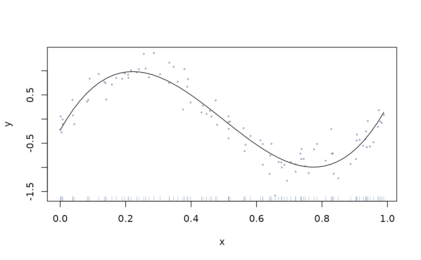
data_rug: logical; when TRUE, draw rug-style support cues for the plotted coordinates. For ordinary one-dimensional base plots this behaves like a standard rug. For eligible bivariate surface plots, the base renderer draws floor-rug ticks and renderer="rgl" draws analogous 3D floor-rug ticks.
legend: legend control for legends drawn by the package, including band="all" uncertainty legends. TRUE draws the default legend, FALSE, NULL, or NA suppresses it, a single character string supplies the legend position, and a list is merged into the default legend call for base plots or the default rgl::legend3d() call for renderer="rgl". For routes with more than one package-drawn legend, named sublists such as legend=list(bands=FALSE) may be used when a route distinguishes those legend roles.
perspective: logical; whether two-continuous-predictor CRS fits should be displayed as bivariate fitted-function surfaces.
phi, theta, view: view controls for bivariate continuous surface plots. As in np, the rgl backend remaps the inherited base defaults theta=0, phi=20 to a more informative oblique view.
renderer: the surface-rendering backend for eligible bivariate continuous plots. "base" uses persp-style graphics. "rgl" uses the suggested rgl package and displays through the active rgl backend. On supported surface routes, data_overlay=TRUE adds observed data as an interactive point cloud, data_rug=TRUE adds 3D floor-rug ticks, and errors!="none" adds interval surfaces. With band="all", CRS draws a matching interactive legend using rgl::legend3d().

Graphical parameters

border, cex, cex.axis, cex.lab, cex.main, cex.sub, col, lty, lwd, main, pch, sub, type, xlab, xlim, ylab, ylim, zlab, zlim: standard graphical controls forwarded to the underlying plotting primitives when relevant.
rgl.persp3d.<arg>, rgl.view3d.<arg>, rgl.par3d.<arg>, rgl.grid3d.<arg>, rgl.widget.<arg>, rgl.surface3d.<arg>, rgl.legend3d.<arg>: backend-specific rgl controls. For example, rgl.legend3d.bty="o" restores a box around the band="all" rgl legend, and rgl.surface3d.alpha customizes interval-surface transparency.

Additional Arguments

Further plotting controls are passed through ... to the relevant plot route.

...: for plot.crs, additional arguments supplied to control plotting behavior or passed through to underlying plotting helpers where supported. Supported named plotting controls are summarized above; standard graphical parameters are forwarded where relevant. For crs_boot_control(), unsupported helper options fail fast rather than being silently ignored.

Details

The default display is the fitted function, matching the modern np regression plot convention. One-dimensional fits are shown as partial fitted curves. For two continuous predictors, perspective=TRUE requests a fitted surface.

Plot interval/error types are:


  "pmzsd"        : point estimate +/- z_(1-alpha/2) * standard error
  "pointwise"    : per-point two-sided interval
  "bonferroni"   : pointwise interval with alpha adjusted for m grid points
  "simultaneous" : joint-band interval from the bootstrap route

where \(m\) is the number of evaluation points used in the plotted curve or surface. band="all" overlays pointwise, simultaneous, and Bonferroni bands.

For mean-regression plots, errors="bootstrap" defaults to the fast fixed-design wild bootstrap used by np, with bootstrap="wild" and B=1999. The refit bootstrap remains available with bootstrap="inid". Mean plots also support the np-style block refit bootstraps bootstrap="fixed" and bootstrap="geom"; use crs_boot_control(blocklen=...) to set the block length explicitly, otherwise the np automatic block-length selector is used.

Quantile CRS plots, i.e. objects fit with tau, follow the npqreg convention and default to the refit bootstrap="inid" selector. bootstrap="fixed" and bootstrap="geom" are also available for quantile fitted-curve plots, while bootstrap="wild" remains mean-only.

For mean CRS gradient/effect plots requested with gradients=TRUE, errors="bootstrap" also defaults to the fixed-design wild bootstrap. Numeric continuous panels report derivative intervals computed with the corresponding crshat() derivative operator. Categorical panels report focal-minus-baseline effect intervals. Refit gradient/effect bootstrap intervals remain available with bootstrap="inid", bootstrap="fixed", and bootstrap="geom". For quantile CRS gradient plots, bootstrap="wild" is not available because quantile estimation is not linear in the response.

Unsupported legacy CRS plot arguments such as ci, deriv, and mean now fail fast. New public plot controls use the np-style names documented here.

Value

Invisibly returns the plotted object for ordinary plotting calls. When output="data" or output="both" is requested, returns the plotting payload. The control helper constructors return small S3 lists consumed by plot.crs() and related CRS plot methods.

Author

Jeffrey S. Racine racinej@mcmaster.ca

Examples

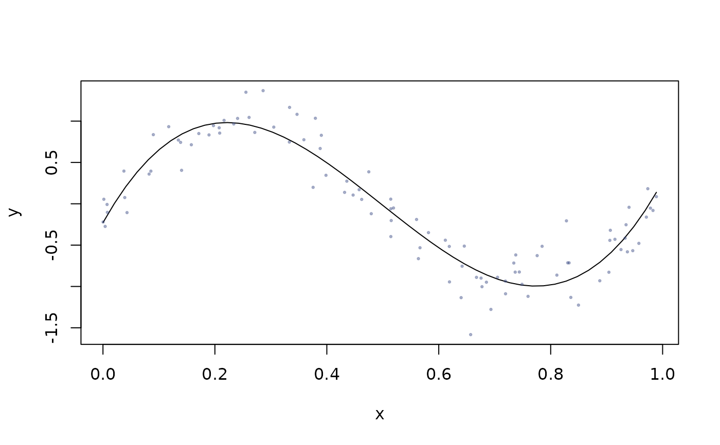
set.seed(42)
n <- 100
x <- runif(n)
y <- sin(2*pi*x) + rnorm(n, sd = 0.25)
model <- crs(y ~ x, cv = "none", degree = 3, segments = 1)

plot(model)

plot(model, data_rug = TRUE)


if (FALSE) { # \dontrun{
plot(model, errors = "bootstrap", band = "all")
plot(model, errors = "bootstrap", bootstrap = "inid", B = 99)
plot(model, errors = "bootstrap", bootstrap = "fixed", B = 99,
     boot_control = crs_boot_control(blocklen = 5))

z <- runif(n)
y2 <- sin(2*pi*x) + z + rnorm(n, sd = 0.25)
smodel <- crs(y2 ~ x + z, cv = "none", degree = c(3, 1),
              segments = c(1, 1))
plot(smodel, perspective = TRUE, data_rug = TRUE)
plot(smodel, perspective = TRUE, renderer = "rgl",
     errors = "bootstrap", band = "all", B = 99)

qmodel <- crs(y ~ x, cv = "none", degree = 3, segments = 1, tau = 0.5)
plot(qmodel, errors = "bootstrap", B = 99)
} # }