Categorical Regression Splines

crs computes a regression spline estimate of a one (1) dimensional dependent variable on an r-dimensional vector of continuous and categorical (factor/ordered) predictors (Ma and Racine (2013), Ma, Racine and Yang (2015)).

Usage

crs(...)
# Default S3 method
crs(xz,
    y,
    basis = c("auto","additive","tensor","glp"),
    complexity = c("degree-knots","degree","knots"),
    data.return = FALSE,
    degree = NULL,
    deriv = 0,
    display.nomad.progress = TRUE,
    display.warnings = TRUE,
    include = NULL,
    kernel = TRUE,
    knots = c("quantiles","uniform","auto"),
    lambda = NULL,
    model.return = FALSE,
    prune = FALSE,
    segments = NULL,
    tau = NULL,
    weights = NULL,
    ...)

# S3 method for class 'formula'
crs(formula,
    basis = c("auto","additive","tensor","glp"),
    complexity = c("degree-knots","degree","knots"),
    cv = c("nomad","exhaustive","none"),
    cv.df.min = 1,
    cv.func = c("cv.ls","cv.gcv","cv.aic"),
    cv.threshold = 1000,
    data = list(),
    data.return = FALSE,
    degree = NULL,
    degree.max = 10,
    degree.min = 0,
    deriv = 0,
    display.nomad.progress = TRUE,
    display.warnings = TRUE,
    include = NULL,
    initial.mesh.size.integer = "1",
    initial.mesh.size.real = "r1.0e-01",
    kernel = TRUE,
    knots = c("quantiles","uniform","auto"),
    lambda = NULL,
    lambda.discrete = FALSE,
    lambda.discrete.num = 100,
    max.bb.eval = NULL,
    max.eval = NULL,
    min.mesh.size.integer = 1,
    min.mesh.size.real = paste(sqrt(.Machine$double.eps)),
    min.frame.size.integer = 1,
    min.frame.size.real = 1,
    model.return = FALSE,
    nmulti = 2,
    opts=list(),
    prune = FALSE,
    random.seed = 42,
    restarts = 0,
    segments = NULL,
    segments.max = 10,
    segments.min = 1,
    singular.ok = FALSE,
    tau = NULL,
    weights = NULL,
    ...)

Arguments

Data, Model Inputs And Formula Interface

These arguments identify the model formula/data interface and explicit data inputs.

data

an optional data frame containing the variables in the model

formula

a symbolic description of the model to be fit

xz

numeric (x) and or nominal/ordinal (factor/ordered) predictors (z)

y

a numeric vector of responses.

Basis, Spline, And Kernel Structure

These arguments control basis type, spline complexity, factor inclusion, and optional kernel smoothing.

basis

a character string (default basis="auto") indicating whether the additive or tensor product B-spline basis matrix for a multivariate polynomial spline or generalized B-spline polynomial basis should be used. Note this can be automatically determined by cross-validation if cv="nomad" or cv="exhaustive" and basis="auto", and is an ‘all or none’ proposition (i.e. interaction terms for all predictors or for no predictors given the nature of ‘tensor products’). Note also that if there is only one predictor this defaults to basis="additive" to avoid unnecessary computation as the spline bases are equivalent in this case

complexity

a character string (default complexity="degree-knots") indicating whether model ‘complexity’ is determined by the degree of the spline or by the number of segments (i.e. number of knots minus one). This option allows the user to use cross-validation to select either the spline degree (number of knots held fixed) or the number of knots (spline degree held fixed) or both the spline degree and number of knots

For the continuous predictors the regression spline model employs either the additive or tensor product B-spline basis matrix for a multivariate polynomial spline via the B-spline routines in the GNU Scientific Library (https://www.gnu.org/software/gsl/) and the tensor.prod.model.matrix function

degree

integer/vector specifying the polynomial degree of the B-spline basis for each dimension of the continuous x (default degree=3, i.e. cubic spline)

degree.max

the maximum degree of the B-spline basis for each of the continuous predictors (default degree.max=10)

degree.min

the minimum degree of the B-spline basis for each of the continuous predictors (default degree.min=0)

include

integer/vector specifying whether each of the nominal/ordinal (factor/ordered) predictors in x are included or omitted from the resulting estimate

kernel

a logical value (default kernel=TRUE) indicating whether to use kernel smoothing or not

knots

a character string (default knots="quantiles") specifying where knots are to be placed. ‘quantiles’ specifies knots placed at equally spaced quantiles (equal number of observations lie in each segment) and ‘uniform’ specifies knots placed at equally spaced intervals. If knots="auto", the knot type will be automatically determined by cross-validation

lambda

a vector of bandwidths for each dimension of the categorical z

lambda.discrete

if lambda.discrete=TRUE, the bandwidth will be discretized into lambda.discrete.num+1 points and lambda will be chosen from these points

lambda.discrete.num

a positive integer indicating the number of discrete values that lambda can assume - this parameter will only be used when lambda.discrete=TRUE

segments

integer/vector specifying the number of segments of the B-spline basis for each dimension of the continuous x (i.e. number of knots minus one) (default segments=1, i.e. Bezier curve)

segments.max

the maximum segments of the B-spline basis for each of the continuous predictors (default segments.max=10)

segments.min

the minimum segments of the B-spline basis for each of the continuous predictors (default segments.min=1)

Cross-Validation And Search Controls

These arguments control cross-validation objective selection and restart behavior.

cv

a character string (default cv="nomad") indicating whether to use nonsmooth mesh adaptive direct search, exhaustive search, or no search (i.e. use user supplied values for degree, segments, and lambda)

cv.df.min

the minimum degrees of freedom to allow when conducting NOMAD-based cross-validation (default cv.df.min=1)

cv.func

a character string (default cv.func="cv.ls") indicating which method to use to select smoothing parameters. cv.gcv specifies generalized cross-validation (Craven and Wahba (1979)), cv.aic specifies expected Kullback-Leibler cross-validation (Hurvich, Simonoff, and Tsai (1998)), and cv.ls specifies least-squares cross-validation

cv.threshold

an integer (default cv.threshold=1000) that controls the automatic switch from NOMAD to exhaustive search for simple problems with no categorical predictors. If cv="nomad" and the number of degree/segments combinations is less than or equal to cv.threshold, crs quietly uses cv="exhaustive" because enumeration is cheap and deterministic. Set cv.threshold=0 to disable this automatic switch and keep cv="nomad" on the NOMAD path. Use cv="exhaustive" to request exhaustive search explicitly.

nmulti

integer number of times to restart the process of finding extrema of the cross-validation function from different (random) initial points (default nmulti=2)

prune

a logical value (default prune=FALSE) specifying whether the (final) model is to be ‘pruned’ using a stepwise cross-validation criterion based upon a modified version of stepAIC (see below for details)

random.seed

when it is not missing and not equal to 0, the initial points will be generated using this seed when using frscvNOMAD or krscvNOMAD and nmulti > 0

restarts

integer specifying the number of times to restart the process of finding extrema of the cross-validation function (for the bandwidths only) from different (random) initial points

singular.ok

a logical value (default singular.ok=FALSE) that, when FALSE, discards singular bases during cross-validation (a check for ill-conditioned bases is performed).

NOMAD Controls

These arguments control NOMAD mesh settings and optional solver controls.

initial.mesh.size.integer

argument passed to the NOMAD solver (see snomadr for further details)

initial.mesh.size.real

argument passed to the NOMAD solver (see snomadr for further details)

max.bb.eval

argument passed to the NOMAD solver. The default NULL lets crs choose a route-specific evaluation budget: 10000 for continuous-only frscvNOMAD search and 1000 for kernel/categorical krscvNOMAD search. These defaults were set on the basis of simulation evidence and real-world applications. User-supplied values are passed through to the selected NOMAD route; see snomadr for further details.

max.eval

optional NOMAD total point-lookup budget. This is distinct from max.bb.eval: max.bb.eval limits true blackbox objective computations, while max.eval limits total NOMAD point lookups, including cache hits. The default NULL uses the selected route's default MAX_EVAL: continuous-only NOMAD search uses MAX_EVAL = 1000, while mixed/kernel NOMAD search retains the historical route behavior of using MAX_BB_EVAL as MAX_EVAL. If supplied, max.eval is passed to NOMAD as MAX_EVAL. Supplying both max.eval and opts$MAX_EVAL with conflicting values is an error.

min.frame.size.integer

arguments passed to the NOMAD solver (see snomadr for further details)

min.frame.size.real

arguments passed to the NOMAD solver (see snomadr for further details)

min.mesh.size.integer

arguments passed to the NOMAD solver (see snomadr for further details)

min.mesh.size.real

argument passed to the NOMAD solver (see snomadr for further details)

opts

list of optional arguments to be passed to snomadr

Quantile, Weights, And Derivatives

These arguments control derivative extraction, quantile level, and observation weights.

deriv

an integer l (default deriv=0) specifying whether to compute the univariate lth partial derivative for each continuous predictor (and difference in levels for each categorical predictor) or not and if so what order. Note that if deriv is higher than the spline degree of the associated continuous predictor then the derivative will be zero and a warning issued to this effect. For predict.crs(), an explicitly supplied deriv= overrides the value stored on the fitted object; when deriv is omitted, prediction preserves the fitted object's derivative setting.

tau

if non-null a number in (0,1) denoting the quantile for which a quantile regression spline is to be estimated rather than estimating the conditional mean (default tau=NULL). Criterion function set by cv.func= are modified accordingly to admit quantile regression.

weights

an optional vector of weights to be used in the fitting process. Should be ‘NULL’ or a numeric vector. If non-NULL, weighted least squares is used with weights ‘weights’ (that is, minimizing ‘sum(w*e^2)’); otherwise ordinary least squares is used.

Returned State And Output Controls

These arguments control whether fitted model state is returned.

data.return

a logical value indicating whether to return x,z,y or not (default data.return=FALSE)

model.return

a logical value indicating whether to return the list of lm models or not when kernel=TRUE (default model.return=FALSE)

Warnings And Progress

These arguments control warnings and displayed optimizer progress.

display.nomad.progress

a logical value indicating whether to display the progress of the NOMAD solver (default display.nomad.progress=TRUE)

display.warnings

a logical value indicating whether to display warnings (default display.warnings=TRUE)

Additional Arguments

Further optional arguments are passed through to lower-level routines.

...

optional arguments

Details

Typical usages are (see below for a list of options and also the examples at the end of this help file)

    ## Estimate the model and let the basis type be determined by
    ## cross-validation (i.e. cross-validation will determine whether to
    ## use the additive, generalized, or tensor product basis)

    model <- crs(y~x1+x2)

    ## Estimate the model for a specified degree/segment/bandwidth
    ## combination and do not run cross-validation (will use the
    ## additive basis by default)

    model <- crs(y~x1+factor(x2),cv="none",degree=3,segments=1,lambda=.1)

    ## Plot the mean and (asymptotic) error bounds

    plot(model,errors = "asymptotic")

    ## Plot the first partial derivative and (asymptotic) error bounds

    plot(model,gradients = TRUE,errors = "asymptotic")
    

crs computes a regression spline estimate of a one (1) dimensional dependent variable on an r-dimensional vector of continuous and categorical (factor/ordered) predictors.

The regression spline model employs the tensor product B-spline basis matrix for a multivariate polynomial spline via the B-spline routines in the GNU Scientific Library (https://www.gnu.org/software/gsl/) and the tensor.prod.model.matrix function.

When basis="additive" the model becomes additive in nature (i.e. no interaction/tensor terms thus semiparametric not fully nonparametric).

When basis="tensor" the model uses the multivariate tensor product basis.

When kernel=FALSE the model uses indicator basis functions for the nominal/ordinal (factor/ordered) predictors rather than kernel weighting.

When kernel=TRUE the product kernel function for the discrete predictors is of the ‘Li-Racine’ type (see Li and Racine (2007) for details).

When cv="nomad", numerical search is undertaken using Nonsmooth Optimization by Mesh Adaptive Direct Search (Abramson, Audet, Couture, Dennis, Jr., and Le Digabel (2011)).

When kernel=TRUE and cv="exhaustive", numerical search is undertaken using optim and the box-constrained L-BFGS-B method (see optim for details). The user may restart the algorithm as many times as desired via the restarts argument (default restarts=0). The approach ascends from degree=0 (or segments=0) through degree.max and for each value of degree (or segments) searches for the optimal bandwidths. After the most complex model has been searched then the optimal degree/segments/lambda combination is selected. If any element of the optimal degree (or segments) vector coincides with degree.max (or segments.max) a warning is produced and the user ought to restart their search with a larger value of degree.max (or segments.max).

Note that the default plot method for a crs object displays the fitted conditional mean or conditional quantile surface. One-dimensional partial fitted curves are drawn by default; for two continuous predictors, perspective=TRUE requests a two-dimensional surface and renderer="rgl" requests the rgl renderer. Surface displays use transparent viridis coloring, NP-style rotation controls via view, and optional data overlays/rugs via data_overlay and data_rug. Gradient displays are requested with gradients=TRUE; higher-order derivatives use gradient_order=i. Intervals are controlled by the modern np-style errors, band, alpha, bootstrap, and B arguments.

Note that setting prune=TRUE produces a final ‘pruning’ of the model via a stepwise cross-validation criterion achieved by modifying stepAIC and replacing extractAIC with extractCV throughout the function. This option may be enabled to remove potentially superfluous bases thereby improving the finite-sample efficiency of the resulting model. Note that if the cross-validation score for the pruned model is no better than that for the original model then the original model is returned with a warning to this effect. Note also that this option can only be used when kernel=FALSE.

Value

crs returns a crs object. The generic functions fitted and residuals extract (or generate) estimated values and residuals. Furthermore, the functions summary, predict, and plot support objects of this type. The plot.crs method follows the modern np plotting interface, including errors=c("none","asymptotic","bootstrap"), gradients=TRUE, gradient_order, output=c("plot","data","plot-data","both"), perspective, renderer, view, neval, band, alpha, bootstrap, B, and the control helpers documented in plot.crs. predict.crs() honors explicit deriv= requests for new evaluation data and, when newdata is omitted, computes explicit derivative requests at the training data; ordinary predict(object) calls retain the stored fitted-value behavior. The returned object has the following components:

fitted.values

estimates of the regression function (conditional mean) at the sample points or evaluation points

lwr,upr

lower/upper bound for a 95% confidence interval for the fitted.values (conditional mean) obtained from predict.lm via the argument interval="confidence". When plotting with errors = "bootstrap", bootstrap-based bounds are used instead for mean plots, including one-dimensional fitted curves and two-dimensional fitted surfaces. Mean-regression plots default to the fast fixed-design wild bootstrap (bootstrap="wild", B=1999) following the modern np interface; the legacy refit bootstrap remains available with bootstrap="inid", and np-style block refit bootstraps are available with bootstrap="fixed" and bootstrap="geom". Quantile CRS plots fit with tau follow the npqreg convention and default to the refit bootstrap="inid" selector; fixed and geom are available for quantile fitted curves, while wild remains mean-only. Mean CRS gradient/effect plots requested with gradients=TRUE also support bootstrap derivative/effect intervals; numeric continuous panels use the corresponding crshat() derivative operator, and categorical panels use focal-minus-baseline effect operators.

residuals

residuals computed at the sample points or evaluation points

degree

integer/vector specifying the degree of the B-spline basis for each dimension of the continuous x

segments

integer/vector specifying the number of segments of the B-spline basis for each dimension of the continuous x

include

integer/vector specifying whether each of the nominal/ordinal (factor/ordered) predictors z are included or omitted from the resulting estimate if kernel=FALSE (see below)

kernel

a logical value indicating whether kernel smoothing was used (kernel=TRUE) or not

lambda

vector of bandwidths used if kernel=TRUE

nomad.summary

summary of NOMAD blackbox evaluations, cache activity, and effective NOMAD options, present only when NOMAD search was used

call

a symbolic description of the model

r.squared

coefficient of determination (Doksum and Samarov (1995))

model.lm

an object of ‘class’ ‘lm’ if kernel=FALSE or a list of objects of ‘class’ ‘lm’ if kernel=TRUE (accessed by model.lm[[1]], model.lm[[2]],...,. By way of example, if foo is a crs object and kernel=FALSE, then foo$model.lm is an object of ‘class’ ‘lm’, while objects of ‘class’ ‘lm’ return the model.frame in model.lm$model which can be accessed via foo$model.lm$model where foo is the crs object (the model frame foo$model.lm$model contains the B-spline bases underlying the estimate which might be of interest). Again by way of example, when kernel=TRUE then foo$model.lm[[1]]$model contains the model frame for the first unique combination of categorical predictors, foo$model.lm[[2]]$model the second and so forth (the weights will potentially differ for each model depending on the value(s) of lambda)

deriv.mat

a matrix of derivatives (or differences in levels for the categorical z) whose order is determined by deriv= in the crs call

deriv.mat.lwr

a matrix of 95% coverage lower bounds for deriv.mat

deriv.mat.upr

a matrix of 95% coverage upper bounds for deriv.mat

hatvalues

the hatvalues for the estimated model

P.hat

the kernel probability estimates corresponding to the categorical predictors in the estimated model

Usage Issues

Note that when kernel=FALSE summary supports the option sigtest=TRUE that conducts an F-test for significance for each predictor.

References

Abramson, M.A. and C. Audet and G. Couture and J.E. Dennis Jr. and and S. Le Digabel (2011), “The NOMAD project”. Software available at https://www.gerad.ca/nomad.

Craven, P. and G. Wahba (1979), “Smoothing Noisy Data With Spline Functions,” Numerische Mathematik, 13, 377-403.

Doksum, K. and A. Samarov (1995), “Nonparametric Estimation of Global Functionals and a Measure of the Explanatory Power of Covariates in Regression,” The Annals of Statistics, 23 1443-1473.

Hurvich, C.M. and J.S. Simonoff and C.L. Tsai (1998), “Smoothing Parameter Selection in Nonparametric Regression Using an Improved Akaike Information Criterion,” Journal of the Royal Statistical Society B, 60, 271-293.

Le Digabel, S. (2011), “Algorithm 909: NOMAD: Nonlinear Optimization With The MADS Algorithm”. ACM Transactions on Mathematical Software, 37(4):44:1-44:15.

Li, Q. and J.S. Racine (2007), Nonparametric Econometrics: Theory and Practice, Princeton University Press.

Ma, S. and J.S. Racine and L. Yang (2015), “Spline Regression in the Presence of Categorical Predictors,” Journal of Applied Econometrics, Volume 30, 705-717.

Ma, S. and J.S. Racine (2013), “Additive Regression Splines with Irrelevant Categorical and Continuous Regressors,” Statistica Sinica, Volume 23, 515-541.

Racine, J.S. (2011), “Cross-Validated Quantile Regression Splines,” manuscript.

Author

Jeffrey S. Racine racinej@mcmaster.ca

See also

smooth.spline, loess, npreg

Examples

set.seed(42)
## Example - simulated data
n <- 1000
num.eval <- 50
x1 <- runif(n)
x2 <- runif(n)
z <- rbinom(n,1,.5)
dgp <- cos(2*pi*x1)+sin(2*pi*x2)+z
z <- factor(z)
y <- dgp + rnorm(n,sd=.5)

## Estimate a model with specified degree, segments, and bandwidth
model <- crs(y~x1+x2+z,degree=c(5,5),
                       segments=c(1,1),
                       lambda=0.1,
                       cv="none",
                       kernel=TRUE)
#> Warning:  cv="none" selected, basis="auto" changed to basis="additive": you might consider basis="tensor" etc.
summary(model)
#> Call:
#> crs.formula(formula = y ~ x1 + x2 + z, cv = "none", degree = c(5, 
#>     5), kernel = TRUE, lambda = 0.1, segments = c(1, 1))
#> 
#> Kernel Weighting/B-spline Bases Regression Spline
#> 
#> There are 2 continuous predictors
#> There is 1 categorical predictor
#> Spline degree/number of segments for x1: 5/1
#> Spline degree/number of segments for x2: 5/1
#> Bandwidth for z: 0.1
#> Model complexity proxy: degree-knots
#> Knot type: quantiles
#> Basis type: additive
#> Training observations: 1000
#> Rank of model frame: 11
#> Trace of smoother matrix: 20
#> 
#> Residual standard error: 0.5057 on 989 degrees of freedom
#> Multiple R-squared: 0.8431,   Adjusted R-squared: 0.8415
#> F-statistic: 275.7 on 19 and 980 DF, p-value: < 2.2e-16
#> Estimation time: 0.0 seconds
#> 

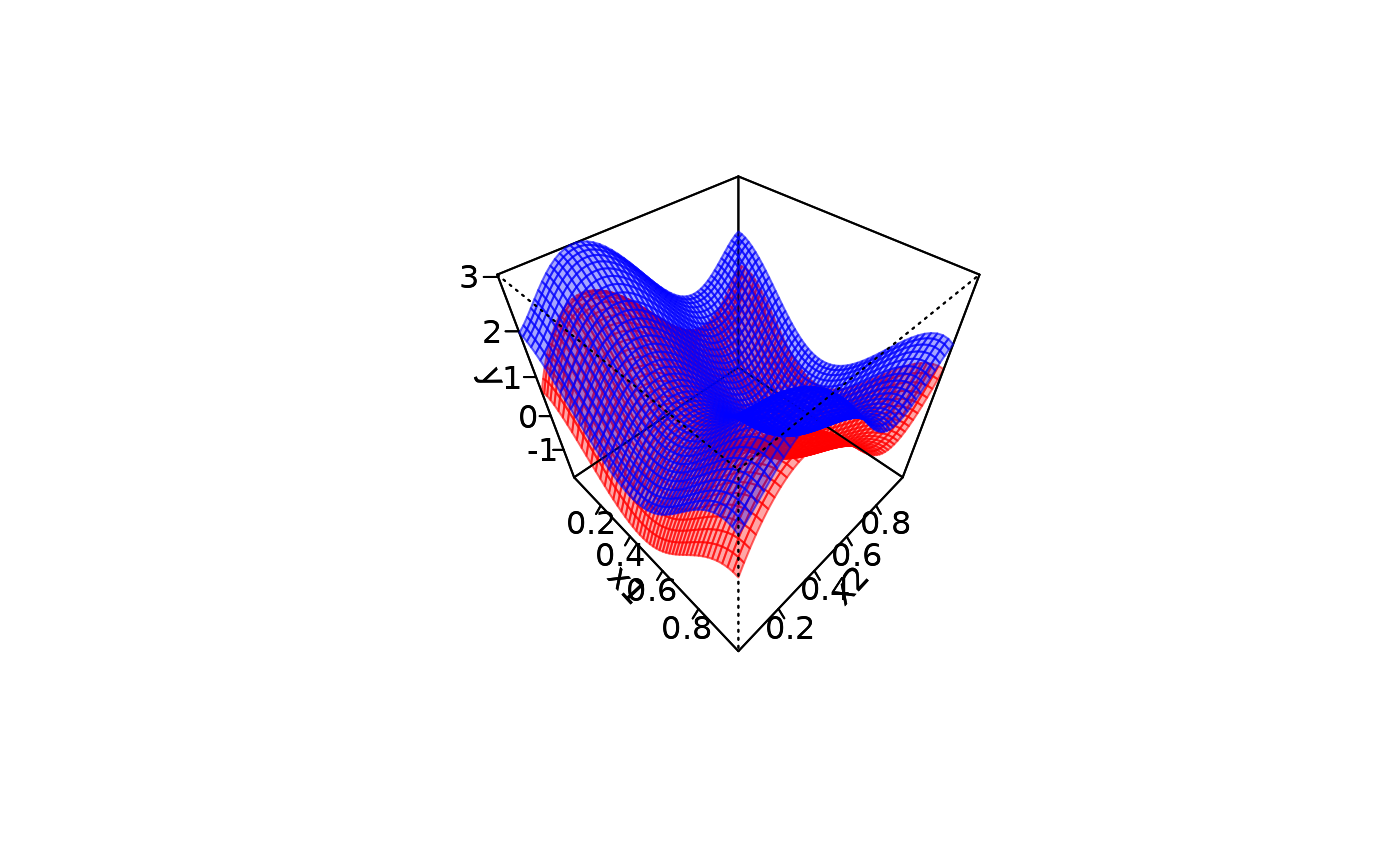
## Perspective plot
x1.seq <- seq(min(x1),max(x1),length=num.eval)
x2.seq <- seq(min(x2),max(x2),length=num.eval)
x.grid <- expand.grid(x1.seq,x2.seq)
newdata <- data.frame(x1=x.grid[,1],x2=x.grid[,2],
                      z=factor(rep(0,num.eval**2),levels=c(0,1)))
z0 <- matrix(predict(model,newdata=newdata),num.eval,num.eval)
newdata <- data.frame(x1=x.grid[,1],x2=x.grid[,2],
                      z=factor(rep(1,num.eval**2),levels=c(0,1)))
z1 <- matrix(predict(model,newdata=newdata),num.eval,num.eval)
zlim=c(min(z0,z1),max(z0,z1))
persp(x=x1.seq,y=x2.seq,z=z0,
      xlab="x1",ylab="x2",zlab="y",zlim=zlim,
      col=grDevices::adjustcolor("red",alpha.f=0.35),
      border=grDevices::adjustcolor("red",alpha.f=0.60),
      ticktype="detailed",
      theta=45,phi=45)
par(new=TRUE)
persp(x=x1.seq,y=x2.seq,z=z1,
      xlab="x1",ylab="x2",zlab="y",zlim=zlim,
      col=grDevices::adjustcolor("blue",alpha.f=0.35),
      border=grDevices::adjustcolor("blue",alpha.f=0.60),
      theta=45,phi=45,
      ticktype="detailed")


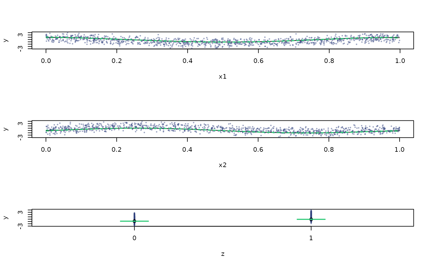
## Partial regression surface plot
plot(model,errors = "asymptotic")

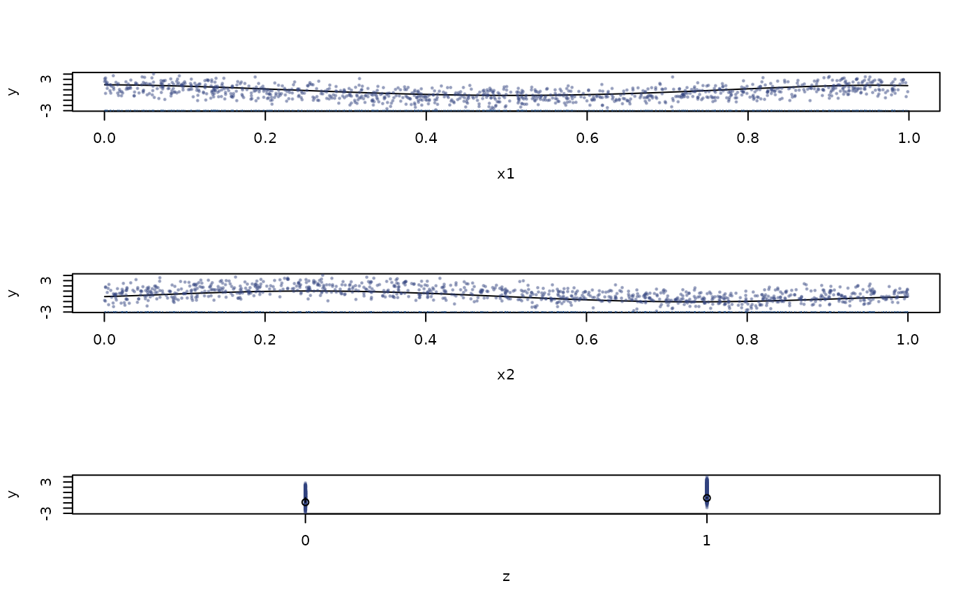
## NP-style data overlay and support rug
plot(model,data_rug=TRUE)

## For two continuous predictors, surface intervals are available through the
## same errors interface
## plot(crs(y~x1+x2,cv="none"),perspective=TRUE,errors="bootstrap",B=99)
## plot(crs(y~x1+x2,cv="none"),perspective=TRUE,renderer="rgl",data_rug=TRUE)
if (FALSE) { # \dontrun{
## A plot example where we extract the partial surfaces, confidence
## intervals etc. automatically generated by plot(...) but do
## not plot, rather save for separate use.
pdat <- plot(model,errors = "asymptotic",output ="data")

## Column 1 is the (evaluation) predictor ([,1]), 2-4 ([,-1]) the mean,
## lwr, and upr (note the returned value is a 'list' hence pdat[[1]] is
## data for the first predictor, pdat[[2]] the second etc). Note that
## matplot() can plot this nicely.
matplot(pdat[[1]][,1],pdat[[1]][,-1],
        xlab=names(pdat[[1]][1]),ylab=names(pdat[[1]][2]),
        lty=c(1,2,2),col=c(1,2,2),type="l")
} # }