A Physiological Model of Unbalanced Algal Growth
aquaphy.RdA phytoplankton model with uncoupled carbon and nitrogen assimilation as a function of light and Dissolved Inorganic Nitrogen (DIN) concentration.
Algal biomass is described via 3 different state variables:
low molecular weight carbohydrates (LMW), the product of photosynthesis,
storage molecules (RESERVE) and
the biosynthetic and photosynthetic apparatus (PROTEINS).
All algal state variables are expressed in \(\rm mmol\, C\, m^{-3}\). Only proteins contain nitrogen and chlorophyll, with a fixed stoichiometric ratio. As the relative amount of proteins changes in the algae, so does the N:C and the Chl:C ratio.
An additional state variable, dissolved inorganic nitrogen (DIN) has units of \(\rm mmol\, N\, m^{-3}\).
The algae grow in a dilution culture (chemostat): there is constant inflow of DIN and outflow of culture water, including DIN and algae, at the same rate.
Two versions of the model are included.
In the default model, there is a day-night illumination regime, i.e. the light is switched on and off at fixed times (where the sum of illuminated + dark period = 24 hours).
In another version, the light is imposed as a forcing function data set.
This model is written in FORTRAN.
aquaphy(times, y, parms, PAR = NULL, ...)Arguments
- times
time sequence for which output is wanted; the first value of times must be the initial time,
- y
the initial (state) values ("DIN", "PROTEIN", "RESERVE", "LMW"), in that order,
- parms
vector or list with the aquaphy model parameters; see the example for the order in which these have to be defined.
- PAR
a data set of the photosynthetically active radiation (light intensity), if
NULL, on-off PAR is used,- ...
any other parameters passed to the integrator
ode(which solves the model).
References
Lancelot, C., Veth, C. and Mathot, S. (1991). Modelling ice-edge phytoplankton bloom in the Scotia-Weddel sea sector of the Southern Ocean during spring 1988. Journal of Marine Systems 2, 333–346.
Soetaert, K. and Herman, P. (2008). A practical guide to ecological modelling. Using R as a simulation platform. Springer.
Details
The model is implemented primarily to demonstrate the linking of FORTRAN with R-code.
The source can be found in the doc/examples/dynload subdirectory of the package.
See also
ccl4model, the CCl4 inhalation model.
Examples
## ======================================================
##
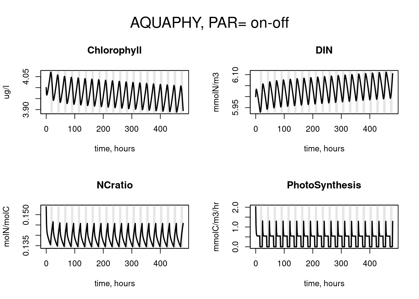
## Example 1. PAR an on-off function
##
## ======================================================
## -----------------------------
## the model parameters:
## -----------------------------
parameters <- c(maxPhotoSynt = 0.125, # mol C/mol C/hr
rMortPHY = 0.001, # /hr
alpha = -0.125/150, # uEinst/m2/s/hr
pExudation = 0.0, # -
maxProteinSynt = 0.136, # mol C/mol C/hr
ksDIN = 1.0, # mmol N/m3
minpLMW = 0.05, # mol C/mol C
maxpLMW = 0.15, # mol C/mol C
minQuotum = 0.075, # mol C/mol C
maxStorage = 0.23, # /h
respirationRate= 0.0001, # /h
pResp = 0.4, # -
catabolismRate = 0.06, # /h
dilutionRate = 0.01, # /h
rNCProtein = 0.2, # mol N/mol C
inputDIN = 10.0, # mmol N/m3
rChlN = 1, # g Chl/mol N
parMean = 250., # umol Phot/m2/s
dayLength = 15. # hours
)
## -----------------------------
## The initial conditions
## -----------------------------
state <- c(DIN = 6., # mmol N/m3
PROTEIN = 20.0, # mmol C/m3
RESERVE = 5.0, # mmol C/m3
LMW = 1.0) # mmol C/m3
## -----------------------------
## Running the model
## -----------------------------
times <- seq(0, 24*20, 1)
out <- as.data.frame(aquaphy(times, state, parameters))
## -----------------------------
## Plotting model output
## -----------------------------
par(mfrow = c(2, 2), oma = c(0, 0, 3, 0))
col <- grey(0.9)
ii <- 1:length(out$PAR)
plot(times[ii], out$Chlorophyll[ii], type = "l",
main = "Chlorophyll", xlab = "time, hours",ylab = "ug/l")
polygon(times[ii], out$PAR[ii]-10, col = col, border = NA); box()
lines(times[ii], out$Chlorophyll[ii], lwd = 2 )
plot (times[ii], out$DIN[ii], type = "l", main = "DIN",
xlab = "time, hours",ylab = "mmolN/m3")
polygon(times[ii], out$PAR[ii]-10, col = col, border = NA); box()
lines(times[ii], out$DIN[ii], lwd = 2 )
plot (times[ii], out$NCratio[ii], type = "n", main = "NCratio",
xlab = "time, hours", ylab = "molN/molC")
polygon(times[ii], out$PAR[ii]-10, col = col, border = NA); box()
lines(times[ii], out$NCratio[ii], lwd = 2 )
plot (times[ii], out$PhotoSynthesis[ii],type = "l",
main = "PhotoSynthesis", xlab = "time, hours",
ylab = "mmolC/m3/hr")
polygon(times[ii], out$PAR[ii]-10, col = col, border = NA); box()
lines(times[ii], out$PhotoSynthesis[ii], lwd = 2 )
mtext(outer = TRUE, side = 3, "AQUAPHY, PAR= on-off", cex = 1.5)
 ## -----------------------------
## Summary model output
## -----------------------------
t(summary(out))
#>
#> time Min. : 0 1st Qu.:120 Median :240
#> DIN Min. :5.929 1st Qu.:5.995 Median :6.029
#> PROTEIN Min. :19.44 1st Qu.:19.67 Median :19.86
#> RESERVE Min. :4.776 1st Qu.:5.197 Median :5.570
#> LMW Min. :1.000 1st Qu.:2.637 Median :3.431
#> PAR Min. : 0.0 1st Qu.: 0.0 Median :250.0
#> TotalN Min. :10 1st Qu.:10 Median :10
#> PhotoSynthesis Min. :0.0000 1st Qu.:0.0000 Median :0.5386
#> NCratio Min. :0.1345 1st Qu.:0.1364 Median :0.1383
#> ChlCratio Min. :0.1345 1st Qu.:0.1364 Median :0.1383
#> Chlorophyll Min. :3.888 1st Qu.:3.935 Median :3.971
#>
#> time Mean :240 3rd Qu.:360 Max. :480
#> DIN Mean :6.029 3rd Qu.:6.065 Max. :6.112
#> PROTEIN Mean :19.85 3rd Qu.:20.03 Max. :20.35
#> RESERVE Mean :5.561 3rd Qu.:5.908 Max. :6.158
#> LMW Mean :3.176 3rd Qu.:3.586 Max. :3.706
#> PAR Mean :156.4 3rd Qu.:250.0 Max. :250.0
#> TotalN Mean :10 3rd Qu.:10 Max. :10
#> PhotoSynthesis Mean :0.3879 3rd Qu.:0.5443 Max. :2.0278
#> NCratio Mean :0.1390 3rd Qu.:0.1418 Max. :0.1538
#> ChlCratio Mean :0.1390 3rd Qu.:0.1418 Max. :0.1538
#> Chlorophyll Mean :3.971 3rd Qu.:4.005 Max. :4.071
## ======================================================
##
## Example 2. PAR a forcing function data set
##
## ======================================================
times <- seq(0, 24*20, 1)
## -----------------------------
## create the forcing functions
## -----------------------------
ftime <- seq(0,500,by=0.5)
parval <- pmax(0,250 + 350*sin(ftime*2*pi/24)+
(runif(length(ftime))-0.5)*250)
Par <- matrix(nc=2,c(ftime,parval))
state <- c(DIN = 6., # mmol N/m3
PROTEIN = 20.0, # mmol C/m3
RESERVE = 5.0, # mmol C/m3
LMW = 1.0) # mmol C/m3
out <- aquaphy(times, state, parameters, Par)
plot(out, which = c("PAR", "Chlorophyll", "DIN", "NCratio"),
xlab = "time, hours",
ylab = c("uEinst/m2/s", "ug/l", "mmolN/m3", "molN/molC"))
mtext(outer = TRUE, side = 3, "AQUAPHY, PAR=forcing", cex = 1.5)
## -----------------------------
## Summary model output
## -----------------------------
t(summary(out))
#>
#> time Min. : 0 1st Qu.:120 Median :240
#> DIN Min. :5.929 1st Qu.:5.995 Median :6.029
#> PROTEIN Min. :19.44 1st Qu.:19.67 Median :19.86
#> RESERVE Min. :4.776 1st Qu.:5.197 Median :5.570
#> LMW Min. :1.000 1st Qu.:2.637 Median :3.431
#> PAR Min. : 0.0 1st Qu.: 0.0 Median :250.0
#> TotalN Min. :10 1st Qu.:10 Median :10
#> PhotoSynthesis Min. :0.0000 1st Qu.:0.0000 Median :0.5386
#> NCratio Min. :0.1345 1st Qu.:0.1364 Median :0.1383
#> ChlCratio Min. :0.1345 1st Qu.:0.1364 Median :0.1383
#> Chlorophyll Min. :3.888 1st Qu.:3.935 Median :3.971
#>
#> time Mean :240 3rd Qu.:360 Max. :480
#> DIN Mean :6.029 3rd Qu.:6.065 Max. :6.112
#> PROTEIN Mean :19.85 3rd Qu.:20.03 Max. :20.35
#> RESERVE Mean :5.561 3rd Qu.:5.908 Max. :6.158
#> LMW Mean :3.176 3rd Qu.:3.586 Max. :3.706
#> PAR Mean :156.4 3rd Qu.:250.0 Max. :250.0
#> TotalN Mean :10 3rd Qu.:10 Max. :10
#> PhotoSynthesis Mean :0.3879 3rd Qu.:0.5443 Max. :2.0278
#> NCratio Mean :0.1390 3rd Qu.:0.1418 Max. :0.1538
#> ChlCratio Mean :0.1390 3rd Qu.:0.1418 Max. :0.1538
#> Chlorophyll Mean :3.971 3rd Qu.:4.005 Max. :4.071
## ======================================================
##
## Example 2. PAR a forcing function data set
##
## ======================================================
times <- seq(0, 24*20, 1)
## -----------------------------
## create the forcing functions
## -----------------------------
ftime <- seq(0,500,by=0.5)
parval <- pmax(0,250 + 350*sin(ftime*2*pi/24)+
(runif(length(ftime))-0.5)*250)
Par <- matrix(nc=2,c(ftime,parval))
state <- c(DIN = 6., # mmol N/m3
PROTEIN = 20.0, # mmol C/m3
RESERVE = 5.0, # mmol C/m3
LMW = 1.0) # mmol C/m3
out <- aquaphy(times, state, parameters, Par)
plot(out, which = c("PAR", "Chlorophyll", "DIN", "NCratio"),
xlab = "time, hours",
ylab = c("uEinst/m2/s", "ug/l", "mmolN/m3", "molN/molC"))
mtext(outer = TRUE, side = 3, "AQUAPHY, PAR=forcing", cex = 1.5)
 # Now all variables plotted in one figure...
plot(out, which = 1:9, type = "l")
#> Warning: axis(2, *): range of values ( 0) is small wrt |M| = 10 --> not pretty()
# Now all variables plotted in one figure...
plot(out, which = 1:9, type = "l")
#> Warning: axis(2, *): range of values ( 0) is small wrt |M| = 10 --> not pretty()
 par(mfrow = c(1, 1))