Kullback-Leibler Divergence — KLdiv • flexmix

Estimate the Kullback-Leibler divergence of several distributions.

# S4 method for class 'matrix'
KLdiv(object, eps = 10^-4, overlap = TRUE,...)
# S4 method for class 'flexmix'
KLdiv(object, method = c("continuous", "discrete"), ...)

Arguments

object: See Methods section below.
method: The method to be used; "continuous" determines the Kullback-Leibler divergence between the unweighted theoretical component distributions and the unweighted posterior probabilities at the observed points are used by "discrete".
eps: Probabilities below this threshold are replaced by this threshold for numerical stability.
overlap: Logical, do not determine the KL divergence for those pairs where for each point at least one of the densities has a value smaller than eps.
...: Passed to the matrix method.

Methods

object = "matrix":: Takes as input a matrix of density values with one row per observation and one column per distribution.
object = "flexmix":: Returns the Kullback-Leibler divergence of the mixture components.

Details

Estimates $$\int f(x) (\log f(x) - \log g(x)) dx$$ for distributions with densities $f()$ and $g()$.

Value

A matrix of KL divergences where the rows correspond to using the respective distribution as $f()$ in the formula above.

Note

The density functions are modified to have equal support. A weight of at least eps is given to each observation point for the modified densities.

Author

Friedrich Leisch and Bettina Gruen

References

S. Kullback and R. A. Leibler. On information and sufficiency.The Annals of Mathematical Statistics, 22(1), 79–86, 1951.

Friedrich Leisch. Exploring the structure of mixture model components. In Jaromir Antoch, editor, Compstat 2004–Proceedings in Computational Statistics, 1405–1412. Physika Verlag, Heidelberg, Germany, 2004. ISBN 3-7908-1554-3.

Examples

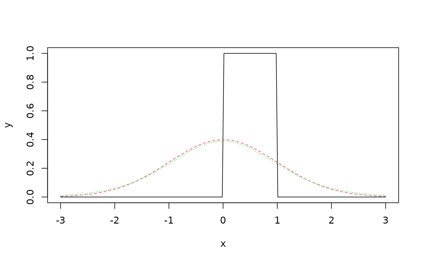
## Gaussian and Student t are much closer to each other than
## to the uniform:

x <- seq(-3, 3, length = 200)
y <- cbind(u = dunif(x), n = dnorm(x), t = dt(x, df = 10))

matplot(x, y, type = "l")

KLdiv(y)
#>          u           n           t
#> u 0.000000 1.082016066 1.107696457
#> n 4.661417 0.000000000 0.004314432
#> t 4.685997 0.005138101 0.000000000

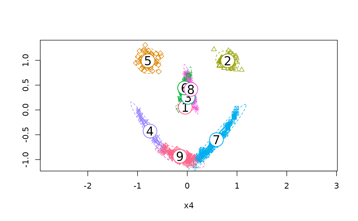
if (require("mlbench")) {
set.seed(2606)
x <-  mlbench.smiley()$x
model1 <- flexmix(x ~ 1, k = 9, model = FLXmclust(diag = FALSE),
                  control  =  list(minprior = 0))
plotEll(model1, x)
KLdiv(model1)
}
#> Loading required package: mlbench

#>            [,1]      [,2]       [,3]       [,4]      [,5]      [,6]       [,7]
#>  [1,]   0.00000 127.38549  10.465786  347.39410  65.96873  15.68134  238.37734
#>  [2,] 355.09493   0.00000 515.453871 2046.99689 124.57769 342.86906  216.96622
#>  [3,]  16.37309  91.53808   0.000000  485.00219  55.37133  11.91903  285.47909
#>  [4,] 135.20050 346.13459 473.194050    0.00000  94.69614 180.33986  401.47033
#>  [5,] 374.62909 141.08019 245.535712  274.52425   0.00000 524.48359 1259.40178
#>  [6,]  63.83343  77.94779   7.378457  538.34468  40.15853   0.00000  394.59000
#>  [7,] 222.54714 214.59542 170.061156  555.34119 206.81012 597.40484    0.00000
#>  [8,]  60.69815  68.54197   7.659784  625.11702  51.71476  19.63367  326.94140
#>  [9,] 352.43050 381.10288 206.550561   34.20101 187.22028 115.71277   49.44981
#>             [,8]      [,9]
#>  [1,]  44.405475 131.53573
#>  [2,] 701.249827 645.13681
#>  [3,]   9.320418 194.35845
#>  [4,] 965.009194  19.41957
#>  [5,] 464.799392 365.19535
#>  [6,]  20.048972 251.81501
#>  [7,] 156.737792  66.82421
#>  [8,]   0.000000 257.36165
#>  [9,] 332.601354   0.00000