Arrange Multiple ggplots

Arrange multiple ggplots on the same page. Wrapper around plot_grid(). Can arrange multiple ggplots over multiple pages, compared to the standard plot_grid(). Can also create a common unique legend for multiple plots.

Usage

ggarrange(
  ...,
  plotlist = NULL,
  ncol = NULL,
  nrow = NULL,
  labels = NULL,
  label.x = 0,
  label.y = 1,
  hjust = -0.5,
  vjust = 1.5,
  font.label = list(size = 14, color = "black", face = "bold", family = NULL),
  align = c("none", "h", "v", "hv"),
  widths = 1,
  heights = 1,
  byrow = TRUE,
  legend = NULL,
  common.legend = FALSE,
  legend.grob = NULL,
  spacing = 0
)

Arguments

...: list of plots to be arranged into the grid. The plots can be either ggplot2 plot objects or arbitrary gtables.
plotlist: (optional) list of plots to display.
ncol: (optional) number of columns in the plot grid.
nrow: (optional) number of rows in the plot grid.
labels: (optional) list of labels to be added to the plots. You can also set labels="AUTO" to auto-generate upper-case labels or labels="auto" to auto-generate lower-case labels.
label.x: (optional) Single value or vector of x positions for plot labels, relative to each subplot. Defaults to 0 for all labels. (Each label is placed all the way to the left of each plot.)
label.y: (optional) Single value or vector of y positions for plot labels, relative to each subplot. Defaults to 1 for all labels. (Each label is placed all the way to the top of each plot.)
hjust: Adjusts the horizontal position of each label. More negative values move the label further to the right on the plot canvas. Can be a single value (applied to all labels) or a vector of values (one for each label). Default is -0.5.
vjust: Adjusts the vertical position of each label. More positive values move the label further down on the plot canvas. Can be a single value (applied to all labels) or a vector of values (one for each label). Default is 1.5.
font.label: a list of arguments for customizing labels. Allowed values are the combination of the following elements: size (e.g.: 14), face (e.g.: "plain", "bold", "italic", "bold.italic"), color (e.g.: "red") and family. For example font.label = list(size = 14, face = "bold", color ="red").
align: (optional) Specifies whether graphs in the grid should be horizontally ("h") or vertically ("v") aligned. Options are "none" (default), "hv" (align in both directions), "h", and "v".
widths: (optional) numerical vector of relative columns widths. For example, in a two-column grid, widths = c(2, 1) would make the first column twice as wide as the second column.
heights: same as widths but for column heights.
byrow: logical. If TRUE (default), the plots are filled into the grid by row; set to FALSE to fill by column. Passed to plot_grid().
legend: character specifying legend position. Allowed values are one of c("top", "bottom", "left", "right", "none"). To remove the legend use legend = "none".
common.legend: logical value, or one or several plot indices. Default is FALSE. If TRUE, a single shared legend is used for all the arranged plots. Note that this legend is not merged or validated across plots: it is simply the legend of the first plot, and the other legends are dropped. It is therefore only correct when every plot shares the same scale (same groups/levels, order and color range). If the first plot's legend is not representative - for example a group is missing in the first plot, or a continuous color scale spans a different range - the shared legend will misrepresent the other plots. In that case you can: (i) give the plots a consistent scale yourself (e.g. scale_fill_manual(limits = ...) or scale_color_continuous(limits = ...)) so a single legend is valid, and/or (ii) choose which plot's legend is shown by passing that plot's index, e.g. common.legend = 2 to use the second plot's legend (equivalent to legend.grob = get_legend(plots[[2]])). You can also pass several indices, e.g. common.legend = c(1, 2), to keep and combine the legends of those plots into a single shared block (side by side for legend = "top"/ "bottom", stacked for "left"/"right") - useful when the plots genuinely need different legends. Note that (ii) only changes which legend is displayed; it does not re-map the other plots' color scales, so for the legend keys to match every panel you still need a consistent scale as in (i). When the plots genuinely cannot be described by a single legend (e.g. a discrete fill in one plot and a continuous color bar in another), use common.legend = FALSE to keep a separate legend per plot.
legend.grob: a legend grob as returned by the function get_legend(). If provided, it will be used as the common legend.
spacing: numeric value giving the margin, in text-line units, set uniformly around each plot to increase the gap between the arranged plots. Default is 0, which leaves each plot's own margins untouched (existing arrangements are unchanged). A positive value sets a uniform margin of that many lines around every plot, replacing the plots' default margin; e.g. spacing = 1 puts a one-line margin around each plot.

Value

an object of class ggarrange, which is a ggplot or a list of ggplots.

Author

Laszlo Erdey erdey.laszlo@econ.unideb.hu

Examples

data("ToothGrowth")
df <- ToothGrowth
df$dose <- as.factor(df$dose)

# Create some plots
# ::::::::::::::::::::::::::::::::::::::::::::::::::
# Box plot
bxp <- ggboxplot(df,
  x = "dose", y = "len",
  color = "dose", palette = "jco"
)
# Dot plot
dp <- ggdotplot(df,
  x = "dose", y = "len",
  color = "dose", palette = "jco"
)
# Density plot
dens <- ggdensity(df, x = "len", fill = "dose", palette = "jco")

# Arrange
# ::::::::::::::::::::::::::::::::::::::::::::::::::
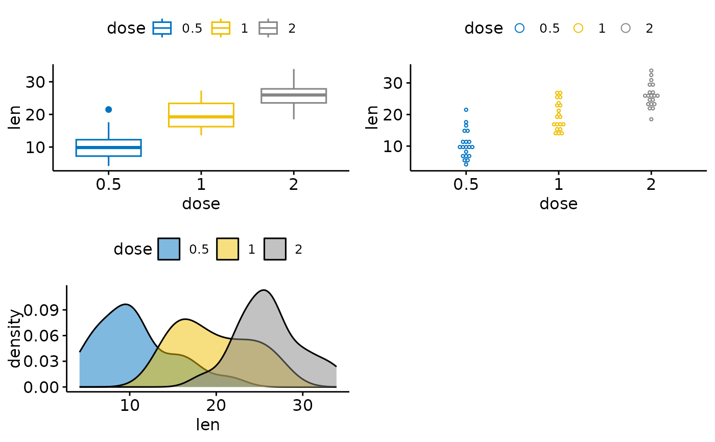
ggarrange(bxp, dp, dens, ncol = 2, nrow = 2)
#> Bin width defaults to 1/30 of the range of the data. Pick better value with
#> `binwidth`.

# Use a common legend for multiple plots
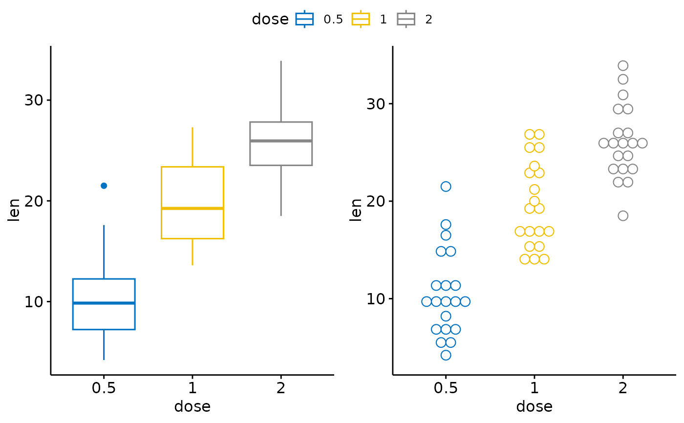
ggarrange(bxp, dp, common.legend = TRUE)
#> Bin width defaults to 1/30 of the range of the data. Pick better value with
#> `binwidth`.

Usage

Arguments

Value

See also

Author

Examples