Add mean comparison p-values to a ggplot, such as box plots, dot plots and stripcharts.
Usage
stat_compare_means(
  mapping = NULL,
  data = NULL,
  method = NULL,
  paired = FALSE,
  id = NULL,
  method.args = list(),
  ref.group = NULL,
  comparisons = NULL,
  hide.ns = FALSE,
  label.sep = ", ",
  label = NULL,
  label.x.npc = "left",
  label.y.npc = "top",
  label.x = NULL,
  label.y = NULL,
  vjust = 0,
  tip.length = 0.03,
  bracket.size = 0.3,
  step.increase = 0,
  symnum.args = list(),
  p.format.style = "default",
  p.digits = NULL,
  p.leading.zero = NULL,
  p.min.threshold = NULL,
  p.decimal.mark = NULL,
  signif.cutoffs = NULL,
  signif.symbols = NULL,
  ns.symbol = "ns",
  use.four.stars = FALSE,
  show.signif = TRUE,
  geom = "text",
  position = "identity",
  na.rm = FALSE,
  show.legend = NA,
  inherit.aes = TRUE,
  ...
)
Arguments
- mapping
Set of aesthetic mappings created by
aes(). If specified andinherit.aes = TRUE(the default), it is combined with the default mapping at the top level of the plot. You must supplymappingif there is no plot mapping.- data
The data to be displayed in this layer. There are three options:
If
NULL, the default, the data is inherited from the plot data as specified in the call toggplot().A
data.frame, or other object, will override the plot data. All objects will be fortified to produce a data frame. Seefortify()for which variables will be created.A
functionwill be called with a single argument, the plot data. The return value must be adata.frame, and will be used as the layer data. Afunctioncan be created from aformula(e.g.~ head(.x, 10)).- method
a character string indicating which method to be used for comparing means.
- paired
a logical indicating whether you want a paired test. Used only in
t.testand in wilcox.test.- id
optional character string naming a column that identifies matched subjects for a paired comparison (
paired = TRUE, withmethod = "t.test"or"wilcox.test", and withoutcomparisons). Without it the paired test pairs observations by row order, so the p-value is wrong when the data are not sorted so that the compared groups align by subject. Providingidpairs the observations by subject id instead (row-order independent); seecompare_means.- method.args
a list of additional arguments used for the test method. For example one might use
method.args = list(alternative = "greater")for wilcoxon test.- ref.group
a character string specifying the reference group. If specified, for a given grouping variable, each of the group levels will be compared to the reference group (i.e. control group).
ref.groupcan be also".all.". In this case, each of the grouping variable levels is compared to all (i.e. basemean).- comparisons
A list of length-2 vectors. The entries in the vector are either the names of 2 values on the x-axis or the 2 integers that correspond to the index of the groups of interest, to be compared.
Note: when
comparisonsis specified, each pairwise test is computed independently and the displayed p-values are not adjusted for multiple comparisons. For p-values corrected for multiple testing, usegeom_pwc(), orstat_pvalue_manual()together withcompare_means(..., p.adjust.method = ).- hide.ns
logical value. If TRUE, hide ns symbol when displaying significance levels.
- label.sep
a character string to separate the terms. Default is ", ", to separate the test method name and the p-value.
- label
character string specifying label type. Allowed values include
"p.signif"(shows the significance levels),"p.format"(shows the formatted p-value), and"p.format.signif"(shows the formatted p-value followed by significance stars, e.g., "p = 0.01 **").- label.x.npc, label.y.npc
can be
numericorcharactervector of the same length as the number of groups and/or panels. If too short they will be recycled.If
numeric, value should be between 0 and 1. Coordinates to be used for positioning the label, expressed in "normalized parent coordinates".If
character, allowed values include: i) one of c('right', 'left', 'center', 'centre', 'middle') for x-axis; ii) and one of c( 'bottom', 'top', 'center', 'centre', 'middle') for y-axis.
- label.x, label.y
numericCoordinates (in data units) to be used for absolute positioning of the label. If too short they will be recycled.- vjust
move the text up or down relative to the bracket.
- tip.length
numeric vector with the fraction that the bracket tips go down to indicate the precise column. Default is 0.03. Can be of same length as the number of comparisons to adjust specifically the tip length of each comparison. For example tip.length = c(0.01, 0.03).
If too short they will be recycled.
Note: when
comparisonsis set, brackets are drawn viaggsignif::geom_signif()andtip.lengthis a fraction of the trained data range, so the absolute tip length scales with your data (plots with different scales get different tip lengths). To obtain visually constant tip lengths across plots, compute the tests withcompare_means()and draw them withstat_pvalue_manual(..., tip.length.ref = "axis")(which makestip.lengtha fraction of the y-axis range). Passingtip.length.refdirectly tostat_compare_means()has no effect and emits an informative message.- bracket.size
Width of the lines of the bracket.
- step.increase
numeric vector with the increase in fraction of total height for every additional comparison to minimize overlap.
- symnum.args
a list of arguments to pass to the function
symnumfor symbolic number coding of p-values. For example,symnum.args <- list(cutpoints = c(0, 0.0001, 0.001, 0.01, 0.05, Inf), symbols = c("****", "***", "**", "*", "ns")).In other words, we use the following convention for symbols indicating statistical significance:
ns: p > 0.05*: p <= 0.05**: p <= 0.01***: p <= 0.001****: p <= 0.0001
Note: If
signif.cutoffsis provided, it takes precedence oversymnum.args.- p.format.style
character string specifying the p-value formatting style. One of:
"default"(backward compatible, uses scientific notation),"apa"(APA style, no leading zero),"nejm"(NEJM style),"lancet"(Lancet style),"ama"(AMA style),"graphpad"(GraphPad style), or"scientific"(scientific notation for GWAS). Seelist_p_format_stylesfor details.- p.digits
integer specifying the number of decimal places for p-values. If provided, overrides the style default.
- p.leading.zero
logical indicating whether to include leading zero before decimal point (e.g., "0.05" vs ".05"). If provided, overrides the style default.
- p.min.threshold
numeric specifying the minimum p-value to display exactly. Values below this threshold are shown as "< threshold". If provided, overrides the style default.
- p.decimal.mark
character string to use as the decimal mark. If NULL, uses
getOption("OutDec").- signif.cutoffs
numeric vector of p-value cutoffs in descending order for assigning significance symbols. For example,
c(0.10, 0.05, 0.01)means p < 0.10 gets "*", p < 0.05 gets "**", p < 0.01 gets "***". Ifuse.four.stars = TRUE, can include a fourth level. Default is NULL, which uses the package defaults.- signif.symbols
character vector of symbols corresponding to
signif.cutoffs. If NULL, auto-generated as "*", "**", "***" (and "****" ifuse.four.stars = TRUE).- ns.symbol
character string for non-significant results. Default is "ns". Use "" (empty string) to show nothing.
- use.four.stars
logical. If TRUE, allows four stars (****) for the most significant level. Default is FALSE.
- show.signif
logical. If TRUE (default), shows significance symbols when using
label = "p.format.signif". If FALSE, falls back to showing only the p-value (equivalent tolabel = "p.format") with a warning.- geom
The geometric object to use to display the data for this layer. When using a
stat_*()function to construct a layer, thegeomargument can be used to override the default coupling between stats and geoms. Thegeomargument accepts the following:A
Geomggproto subclass, for exampleGeomPoint.A string naming the geom. To give the geom as a string, strip the function name of the
geom_prefix. For example, to usegeom_point(), give the geom as"point".For more information and other ways to specify the geom, see the layer geom documentation.
- position
A position adjustment to use on the data for this layer. This can be used in various ways, including to prevent overplotting and improving the display. The
positionargument accepts the following:The result of calling a position function, such as
position_jitter(). This method allows for passing extra arguments to the position.A string naming the position adjustment. To give the position as a string, strip the function name of the
position_prefix. For example, to useposition_jitter(), give the position as"jitter".For more information and other ways to specify the position, see the layer position documentation.
- na.rm
If FALSE (the default), removes missing values with a warning. If TRUE silently removes missing values.
- show.legend
logical. Should this layer be included in the legends?
NA, the default, includes if any aesthetics are mapped.FALSEnever includes, andTRUEalways includes. It can also be a named logical vector to finely select the aesthetics to display. To include legend keys for all levels, even when no data exists, useTRUE. IfNA, all levels are shown in legend, but unobserved levels are omitted.- inherit.aes
If
FALSE(the default for most ggpubr functions), overrides the default aesthetics, rather than combining with them. This is most useful for helper functions that define both data and aesthetics and shouldn't inherit behaviour from the default plot specification. Set toTRUEto inherit aesthetics from the parent ggplot layer.- ...
other arguments to pass to
geom_textorgeom_label.
Details
For grouped plots, if one or more subsets do not contain enough levels to identify the requested comparison, those subsets are skipped and valid subsets are still tested. This avoids fatal layer failures in sparse grouped data settings (Issue #663).
Examples
# Load data
data("ToothGrowth")
head(ToothGrowth)
#> len supp dose
#> 1 4.2 VC 0.5
#> 2 11.5 VC 0.5
#> 3 7.3 VC 0.5
#> 4 5.8 VC 0.5
#> 5 6.4 VC 0.5
#> 6 10.0 VC 0.5
# Two independent groups
# :::::::::::::::::::::::::::::::::::::::::::::::::
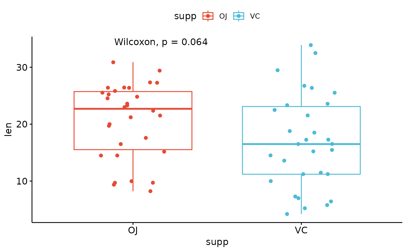
p <- ggboxplot(ToothGrowth,
x = "supp", y = "len",
color = "supp", palette = "npg", add = "jitter"
)
# Add p-value
p + stat_compare_means()
 # Change method
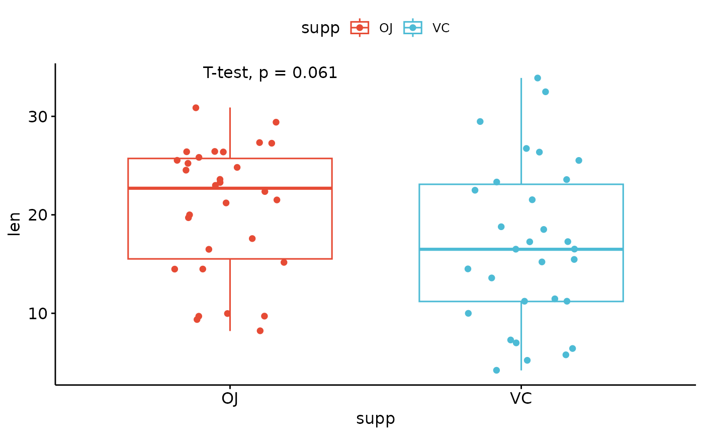
p + stat_compare_means(method = "t.test")
# Change method
p + stat_compare_means(method = "t.test")
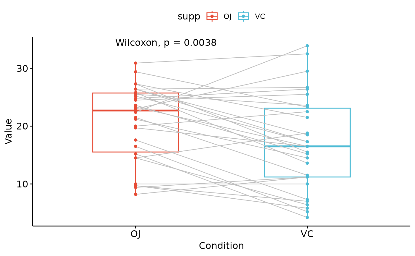
 # Paired samples
# :::::::::::::::::::::::::::::::::::::::::::::::::
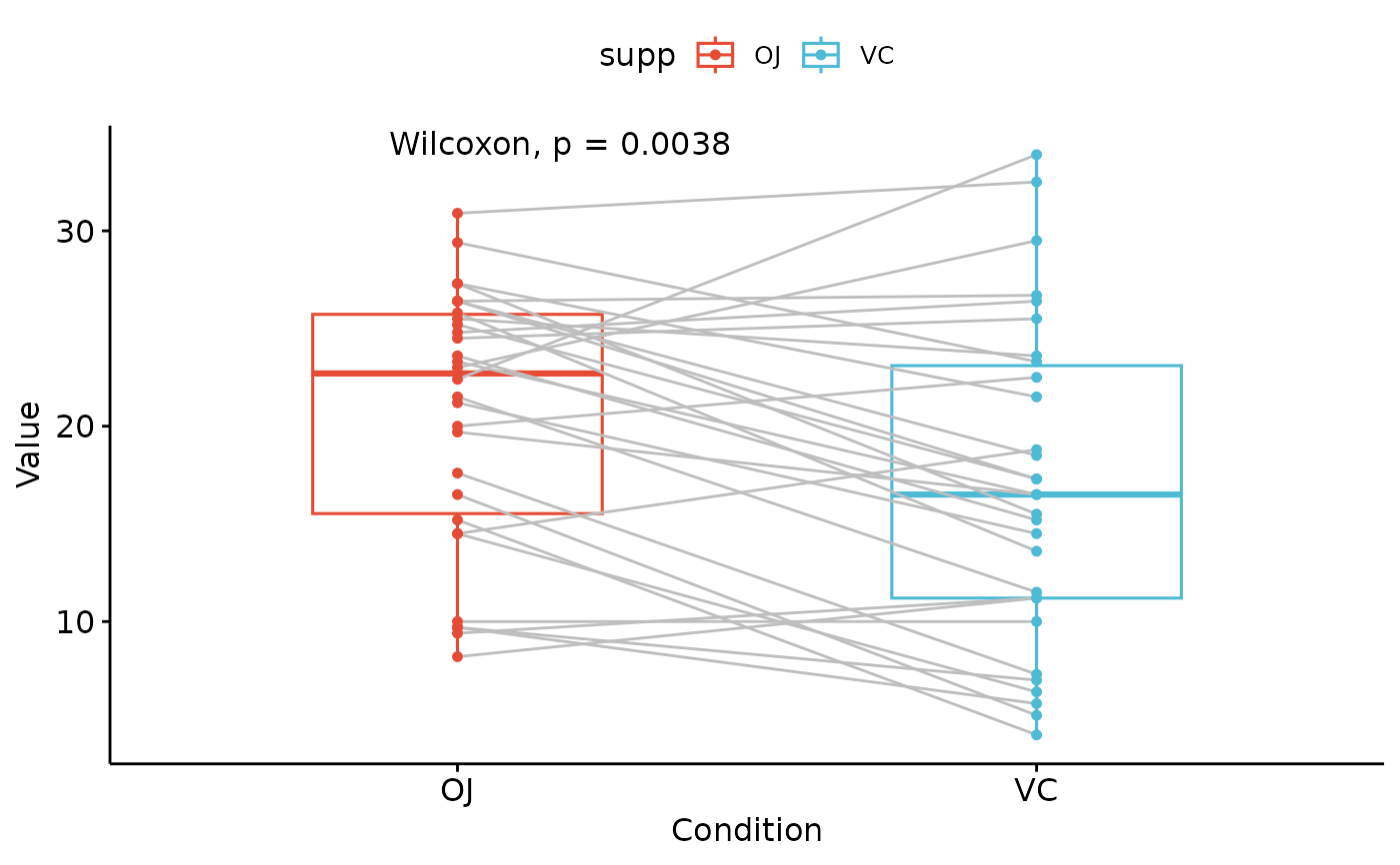
ggpaired(ToothGrowth,
x = "supp", y = "len",
color = "supp", line.color = "gray", line.size = 0.4,
palette = "npg"
) +
stat_compare_means(paired = TRUE)
# Paired samples
# :::::::::::::::::::::::::::::::::::::::::::::::::
ggpaired(ToothGrowth,
x = "supp", y = "len",
color = "supp", line.color = "gray", line.size = 0.4,
palette = "npg"
) +
stat_compare_means(paired = TRUE)
 # Paired samples matched by a subject id column (row-order independent):
# `id` gives the correct p-value even when the rows are not in subject order.
# :::::::::::::::::::::::::::::::::::::::::::::::::
tg <- ToothGrowth
tg$id <- c(1:30, 30:1) # subjects, with the second group in reverse order
ggpaired(tg, x = "supp", y = "len", color = "supp",
line.color = "gray", palette = "npg") +
stat_compare_means(paired = TRUE, id = "id")
# Paired samples matched by a subject id column (row-order independent):
# `id` gives the correct p-value even when the rows are not in subject order.
# :::::::::::::::::::::::::::::::::::::::::::::::::
tg <- ToothGrowth
tg$id <- c(1:30, 30:1) # subjects, with the second group in reverse order
ggpaired(tg, x = "supp", y = "len", color = "supp",
line.color = "gray", palette = "npg") +
stat_compare_means(paired = TRUE, id = "id")
 # More than two groups
# :::::::::::::::::::::::::::::::::::::::::::::::::
# Pairwise comparisons: Specify the comparisons you want
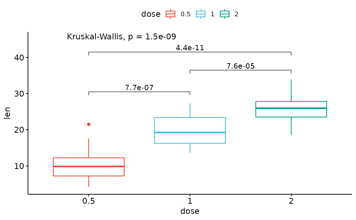
my_comparisons <- list(c("0.5", "1"), c("1", "2"), c("0.5", "2"))
ggboxplot(ToothGrowth,
x = "dose", y = "len",
color = "dose", palette = "npg"
) +
# Add pairwise comparisons p-value
stat_compare_means(comparisons = my_comparisons, label.y = c(29, 35, 40)) +
stat_compare_means(label.y = 45) # Add global Anova p-value
#> `stat_compare_means()` with `comparisons` displays *unadjusted* p-values (no correction for multiple comparisons).
#> ℹ For p-values adjusted for multiple comparisons, use `geom_pwc()`, or `stat_pvalue_manual()` together with `compare_means(..., p.adjust.method = )`.
#> This message is displayed once per session.
# More than two groups
# :::::::::::::::::::::::::::::::::::::::::::::::::
# Pairwise comparisons: Specify the comparisons you want
my_comparisons <- list(c("0.5", "1"), c("1", "2"), c("0.5", "2"))
ggboxplot(ToothGrowth,
x = "dose", y = "len",
color = "dose", palette = "npg"
) +
# Add pairwise comparisons p-value
stat_compare_means(comparisons = my_comparisons, label.y = c(29, 35, 40)) +
stat_compare_means(label.y = 45) # Add global Anova p-value
#> `stat_compare_means()` with `comparisons` displays *unadjusted* p-values (no correction for multiple comparisons).
#> ℹ For p-values adjusted for multiple comparisons, use `geom_pwc()`, or `stat_pvalue_manual()` together with `compare_means(..., p.adjust.method = )`.
#> This message is displayed once per session.
 # Multiple pairwise test against a reference group
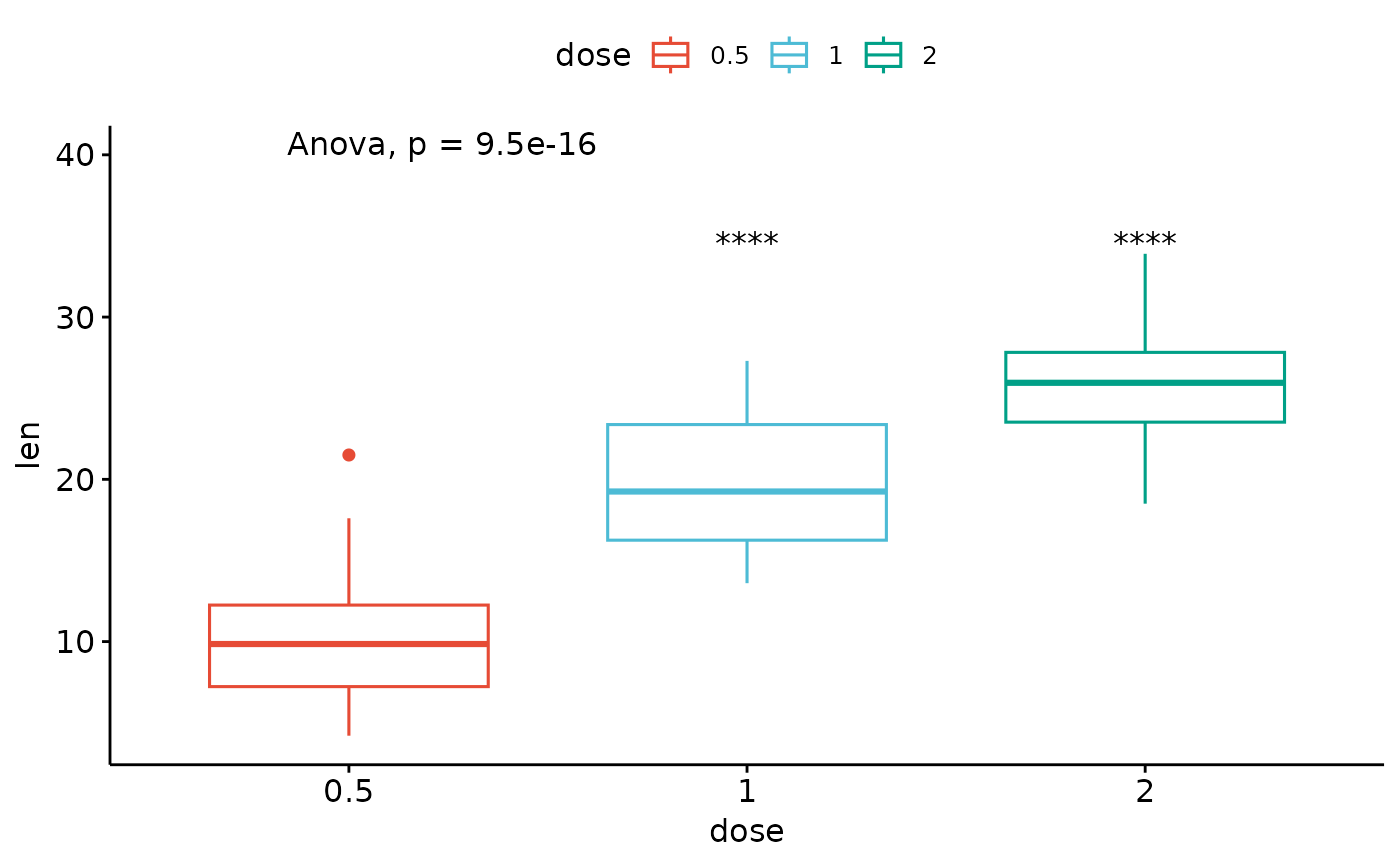
ggboxplot(ToothGrowth,
x = "dose", y = "len",
color = "dose", palette = "npg"
) +
stat_compare_means(method = "anova", label.y = 40) + # Add global p-value
stat_compare_means(aes(label = after_stat(p.signif)),
method = "t.test", ref.group = "0.5"
)
# Multiple pairwise test against a reference group
ggboxplot(ToothGrowth,
x = "dose", y = "len",
color = "dose", palette = "npg"
) +
stat_compare_means(method = "anova", label.y = 40) + # Add global p-value
stat_compare_means(aes(label = after_stat(p.signif)),
method = "t.test", ref.group = "0.5"
)
 # Multiple grouping variables
# :::::::::::::::::::::::::::::::::::::::::::::::::
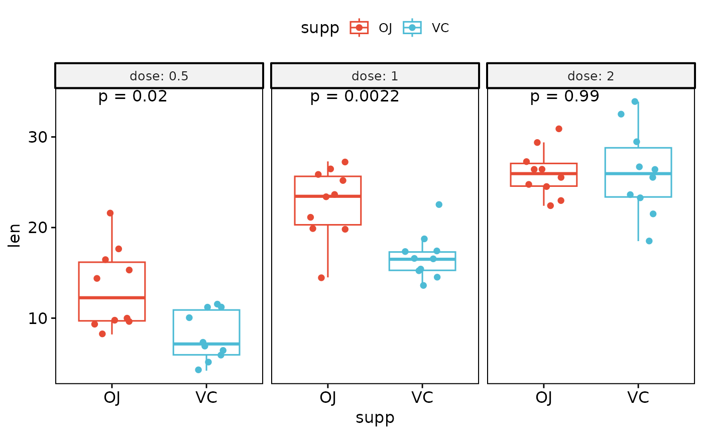
# Box plot facetted by "dose"
p <- ggboxplot(ToothGrowth,
x = "supp", y = "len",
color = "supp", palette = "npg",
add = "jitter",
facet.by = "dose", short.panel.labs = FALSE
)
# Use only p.format as label. Remove method name.
p + stat_compare_means(
aes(label = paste0("p = ", after_stat(p.format)))
)
# Multiple grouping variables
# :::::::::::::::::::::::::::::::::::::::::::::::::
# Box plot facetted by "dose"
p <- ggboxplot(ToothGrowth,
x = "supp", y = "len",
color = "supp", palette = "npg",
add = "jitter",
facet.by = "dose", short.panel.labs = FALSE
)
# Use only p.format as label. Remove method name.
p + stat_compare_means(
aes(label = paste0("p = ", after_stat(p.format)))
)