Add correlation coefficients with p-values to a scatter plot. Can be also used to add `R2`.
Usage
stat_cor(
  mapping = NULL,
  data = NULL,
  method = "pearson",
  alternative = "two.sided",
  cor.coef.name = c("R", "rho", "tau"),
  label.sep = ", ",
  label.x.npc = "left",
  label.y.npc = "top",
  label.x = NULL,
  label.y = NULL,
  label.y.step = 1.4,
  label.anchor = c("data", "panel"),
  output.type = "expression",
  digits = 2,
  r.digits = digits,
  p.digits = digits,
  r.accuracy = NULL,
  p.accuracy = NULL,
  r.leading.zero = NULL,
  p.format.style = "default",
  p.leading.zero = NULL,
  p.decimal.mark = NULL,
  p.coef.name = "p",
  conf.level = 0.95,
  geom = "text",
  position = "identity",
  na.rm = FALSE,
  show.legend = NA,
  inherit.aes = TRUE,
  ...
)
Arguments
- mapping
Set of aesthetic mappings created by
aes(). If specified andinherit.aes = TRUE(the default), it is combined with the default mapping at the top level of the plot. You must supplymappingif there is no plot mapping.- data
The data to be displayed in this layer. There are three options:
If
NULL, the default, the data is inherited from the plot data as specified in the call toggplot().A
data.frame, or other object, will override the plot data. All objects will be fortified to produce a data frame. Seefortify()for which variables will be created.A
functionwill be called with a single argument, the plot data. The return value must be adata.frame, and will be used as the layer data. Afunctioncan be created from aformula(e.g.~ head(.x, 10)).- method
a character string indicating which correlation coefficient (or covariance) is to be computed. One of "pearson" (default), "kendall", or "spearman".
- alternative
a character string specifying the alternative hypothesis, must be one of "two.sided" (default), "greater" or "less". You can specify just the initial letter.
- cor.coef.name
character. Can be one of
"R"(pearson coef),"rho"(spearman coef) and"tau"(kendall coef). Uppercase and lowercase are allowed.- label.sep
a character string to separate the terms. Default is ", ", to separate the correlation coefficient and the p.value.
- label.x.npc, label.y.npc
can be
numericorcharactervector of the same length as the number of groups and/or panels. If too short they will be recycled.If
numeric, value should be between 0 and 1. Coordinates to be used for positioning the label, expressed in "normalized parent coordinates".If
character, allowed values include: i) one of c('right', 'left', 'center', 'centre', 'middle') for x-axis; ii) and one of c( 'bottom', 'top', 'center', 'centre', 'middle') for y-axis.
If too short they will be recycled.
- label.x, label.y
numericCoordinates (in data units) to be used for absolute positioning of the label. If too short they will be recycled.- label.y.step
numeric value giving the vertical spacing (in text-line units) between the labels of successive groups when several groups are present. Default is 1.4 (unchanged behavior). Set
label.y.step = 0to stop the per-group vertical shift, so that labels align across facet panels when a factor is mapped to an aesthetic that also defines the facets. This places the labels flush with the top of each panel; it is similar in spirit to theaes(group = 1)workaround, which instead leaves them one text line lower.- label.anchor
character. How
label.x.npc/label.y.npcare interpreted."data"(default) converts them to data coordinates using the data range, so the label follows the data; the output is unchanged from previous versions."panel"places the label at the true panel-relative position (npc), so the labels stay aligned across panels/facets whose axis ranges differ - e.g. withfacet_wrap(scales = "free_y"), withgeom_smooth()extending each panel by a different amount, or across separate plots combined withggarrange(). An explicitlabel.x/label.yalways stays in data units regardless oflabel.anchor. Requires ggplot2 >= 3.5.0 (already a dependency).- output.type
character One of "expression", "latex", "tex" or "text".
- digits, r.digits, p.digits
integer indicating the number of decimal places (round) or significant digits (signif) to be used for the correlation coefficient and the p-value, respectively. In the default p-value label style, the displayed p-value keeps the legacy raw value unless
p.accuracyis set;p.digitsis used by non-defaultp.format.styleoutputs and the computedpvariable.- r.accuracy
a real value specifying the number of decimal places of precision for the correlation coefficient. Default is NULL. Use (e.g.) 0.01 to show 2 decimal places of precision. If specified, then
r.digitsis ignored.- p.accuracy
a real value specifying the number of decimal places of precision for the p-value. Default is NULL. Use (e.g.) 0.0001 to show 4 decimal places of precision. If specified, then
p.digitsis ignored.- r.leading.zero
logical. Whether to include the leading zero before the decimal point in the correlation coefficient (e.g.,
"0.73"vs".73"). Default (NULL) keeps the leading zero; set toFALSEfor APA-style reporting.- p.format.style
character specifying the p-value formatting style. One of "default", "apa", "nejm", "lancet", "ama", "graphpad", "scientific". Default is "default" for backward compatibility.
- p.leading.zero
logical. Whether to include leading zero before decimal point (e.g., "0.05" vs ".05"). If NULL, uses the style's default setting.
- p.decimal.mark
character string to use as the decimal mark. If NULL, uses
getOption("OutDec").- p.coef.name
character. Symbol used for the p-value label. Default is
"p"; use"P"for an uppercase p-value label. Foroutput.type = "expression"this should be a single valid plotmath symbol (e.g."P"), since it is parsed as an expression.- conf.level
confidence level for the confidence interval of the correlation coefficient, used to compute the
conf.int.low,conf.int.highandconf.int.labelcomputed variables (see the Computed variables section). Default is 0.95. A confidence interval is only available formethod = "pearson"(with at least 4 complete observations); for"spearman"/"kendall"the confidence-interval variables areNA.- geom
The geometric object to use to display the data for this layer. When using a
stat_*()function to construct a layer, thegeomargument can be used to override the default coupling between stats and geoms. Thegeomargument accepts the following:A
Geomggproto subclass, for exampleGeomPoint.A string naming the geom. To give the geom as a string, strip the function name of the
geom_prefix. For example, to usegeom_point(), give the geom as"point".For more information and other ways to specify the geom, see the layer geom documentation.
- position
A position adjustment to use on the data for this layer. This can be used in various ways, including to prevent overplotting and improving the display. The
positionargument accepts the following:The result of calling a position function, such as
position_jitter(). This method allows for passing extra arguments to the position.A string naming the position adjustment. To give the position as a string, strip the function name of the
position_prefix. For example, to useposition_jitter(), give the position as"jitter".For more information and other ways to specify the position, see the layer position documentation.
- na.rm
If FALSE (the default), removes missing values with a warning. If TRUE silently removes missing values.
- show.legend
logical. Should this layer be included in the legends?
NA, the default, includes if any aesthetics are mapped.FALSEnever includes, andTRUEalways includes. It can also be a named logical vector to finely select the aesthetics to display. To include legend keys for all levels, even when no data exists, useTRUE. IfNA, all levels are shown in legend, but unobserved levels are omitted.- inherit.aes
If
FALSE(the default for most ggpubr functions), overrides the default aesthetics, rather than combining with them. This is most useful for helper functions that define both data and aesthetics and shouldn't inherit behaviour from the default plot specification. Set toTRUEto inherit aesthetics from the parent ggplot layer.- ...
other arguments to pass to
geom_textorgeom_label.
Computed variables
- r
correlation coefficient
- rr
correlation coefficient squared
- rmse
root mean square deviation (RMSE/RMSD) between
xandy, computed on the complete pairs; meaningful whenxandyare on the same scale (e.g. predicted vs. reference values). Rounded and formatted with the coefficient settings (r.digits/r.accuracy).- r.label
formatted label for the correlation coefficient
- rr.label
formatted label for the squared correlation coefficient
- p.label
label for the p-value
- rmse.label
formatted label for the RMSE/RMSD
- conf.int.low, conf.int.high
lower and upper bounds of the confidence interval of the correlation coefficient (Pearson only;
NAfor Spearman/Kendall), at the level given byconf.level- conf.int.label
formatted label for the confidence interval, e.g.
"95% CI [0.21, 0.75]"(NAwhen the interval is unavailable)- label
default label displayed by
stat_cor()
See also
ggscatter. For an alternative implementation with more
control over label positioning (native NPC coordinates, per-group vertical and
horizontal steps), see ggpmisc::stat_correlation().
Examples
# Load data
data("mtcars")
df <- mtcars
df$cyl <- as.factor(df$cyl)
# Scatter plot with correlation coefficient
# :::::::::::::::::::::::::::::::::::::::::::::::::
sp <- ggscatter(df,
x = "wt", y = "mpg",
add = "reg.line", # Add regressin line
add.params = list(color = "blue", fill = "lightgray"), # Customize reg. line
conf.int = TRUE # Add confidence interval
)
# Add correlation coefficient
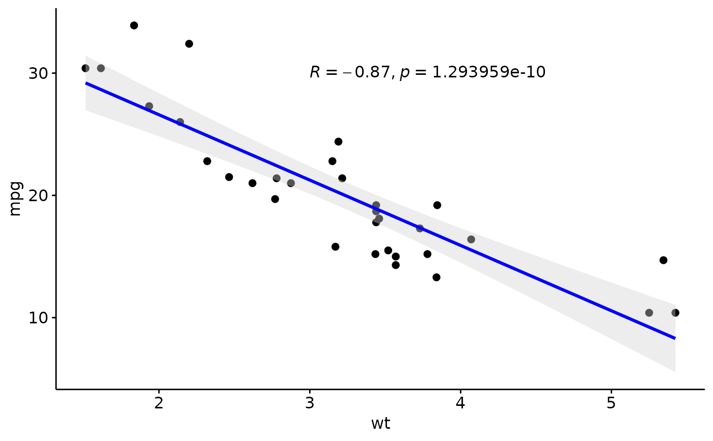
sp + stat_cor(method = "pearson", label.x = 3, label.y = 30)
 # Specify the number of decimal places of precision for p and r
# Using 3 decimal places for the p-value and
# 2 decimal places for the correlation coefficient (r)
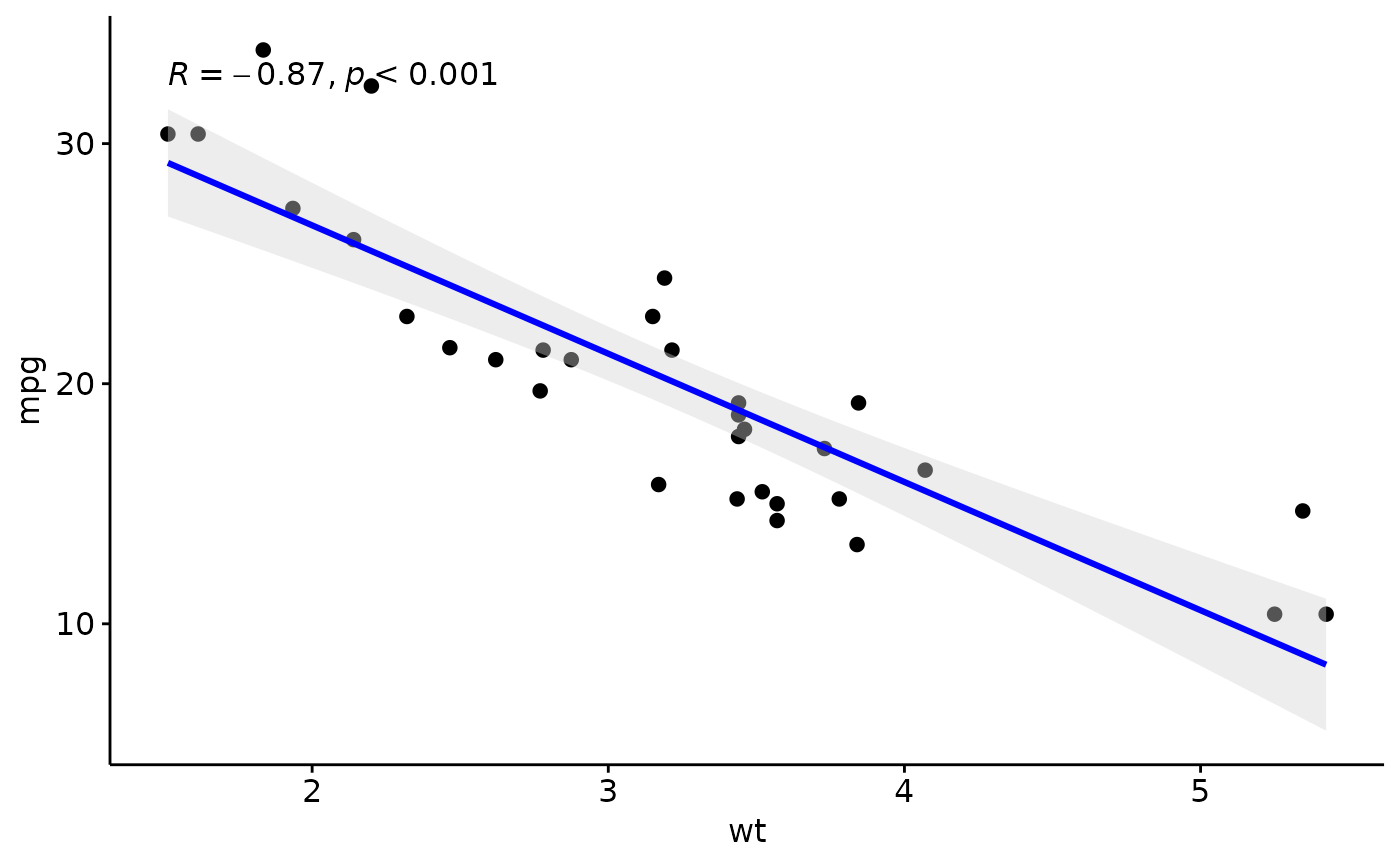
sp + stat_cor(p.accuracy = 0.001, r.accuracy = 0.01)
# Specify the number of decimal places of precision for p and r
# Using 3 decimal places for the p-value and
# 2 decimal places for the correlation coefficient (r)
sp + stat_cor(p.accuracy = 0.001, r.accuracy = 0.01)
 # Show only the r.label but not the p.label
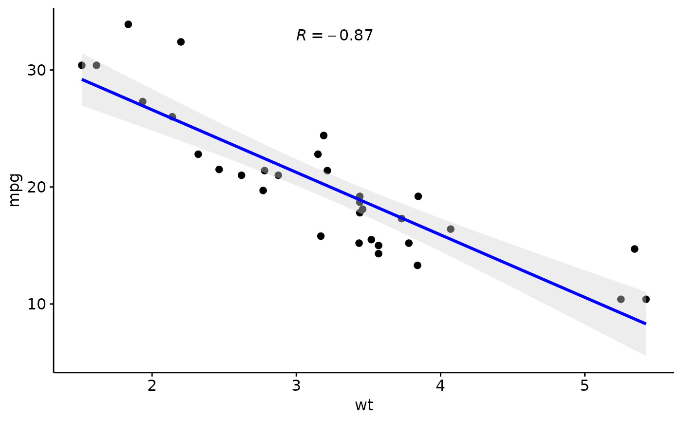
sp + stat_cor(aes(label = after_stat(r.label)), label.x = 3)
# Show only the r.label but not the p.label
sp + stat_cor(aes(label = after_stat(r.label)), label.x = 3)
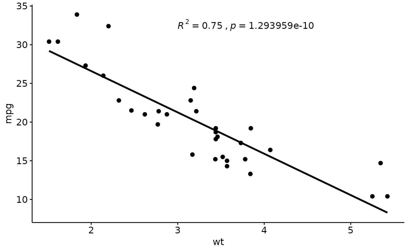
 # Use R2 instead of R
ggscatter(df, x = "wt", y = "mpg", add = "reg.line") +
stat_cor(
aes(label = paste(after_stat(rr.label), after_stat(p.label), sep = "~`,`~")),
label.x = 3
)
# Use R2 instead of R
ggscatter(df, x = "wt", y = "mpg", add = "reg.line") +
stat_cor(
aes(label = paste(after_stat(rr.label), after_stat(p.label), sep = "~`,`~")),
label.x = 3
)
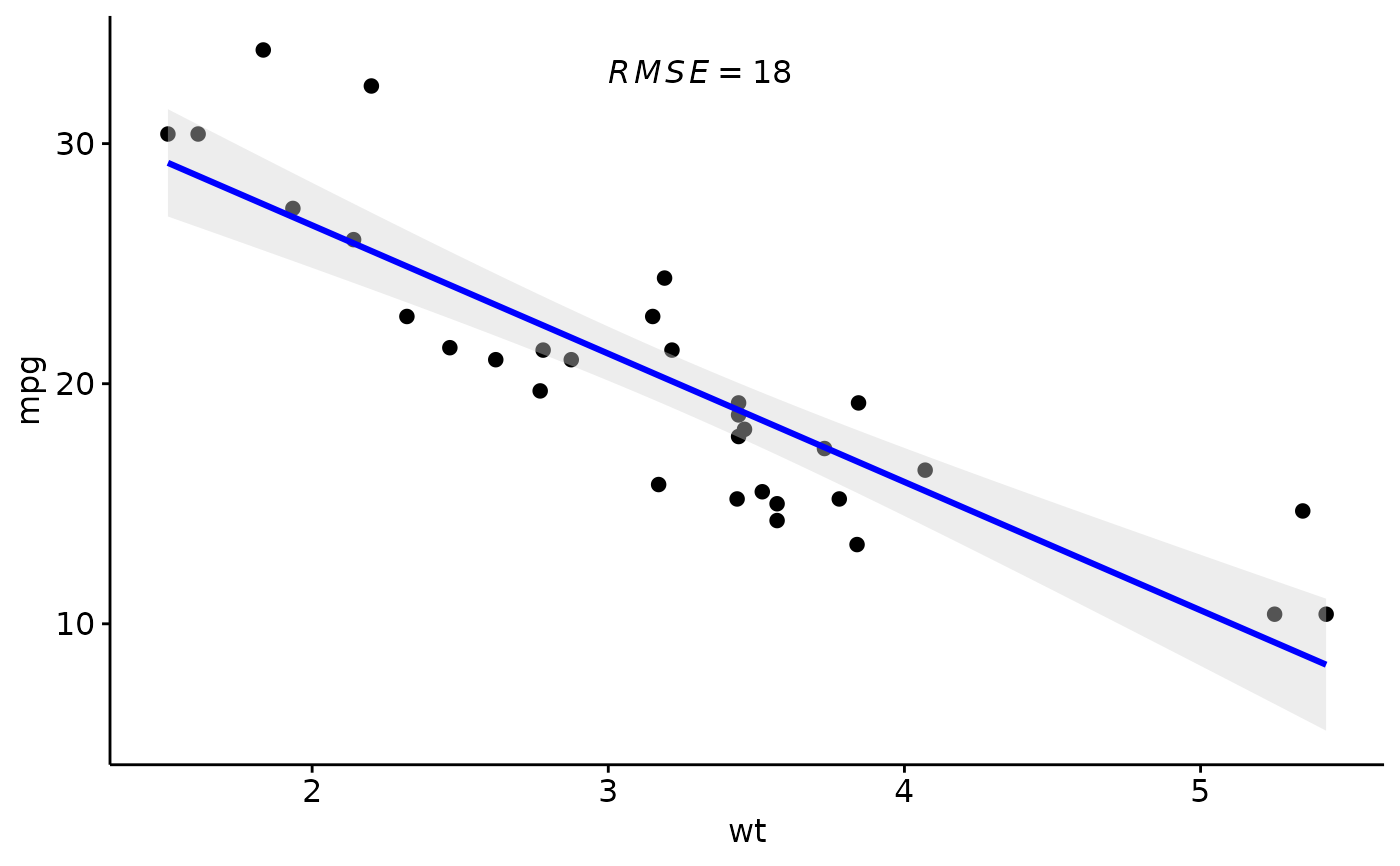
 # Show the RMSE/RMSD (root mean square deviation) between x and y
# (useful for agreement between paired measurements on the same scale)
sp + stat_cor(aes(label = after_stat(rmse.label)), label.x = 3)
# Show the RMSE/RMSD (root mean square deviation) between x and y
# (useful for agreement between paired measurements on the same scale)
sp + stat_cor(aes(label = after_stat(rmse.label)), label.x = 3)
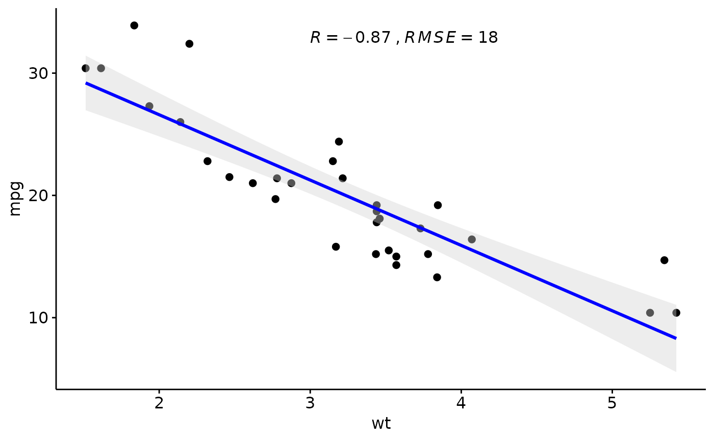
 # Combine the correlation coefficient and the RMSE (comma-separated)
sp + stat_cor(
aes(label = paste(after_stat(r.label), after_stat(rmse.label), sep = "~`,`~")),
label.x = 3
)
# Combine the correlation coefficient and the RMSE (comma-separated)
sp + stat_cor(
aes(label = paste(after_stat(r.label), after_stat(rmse.label), sep = "~`,`~")),
label.x = 3
)
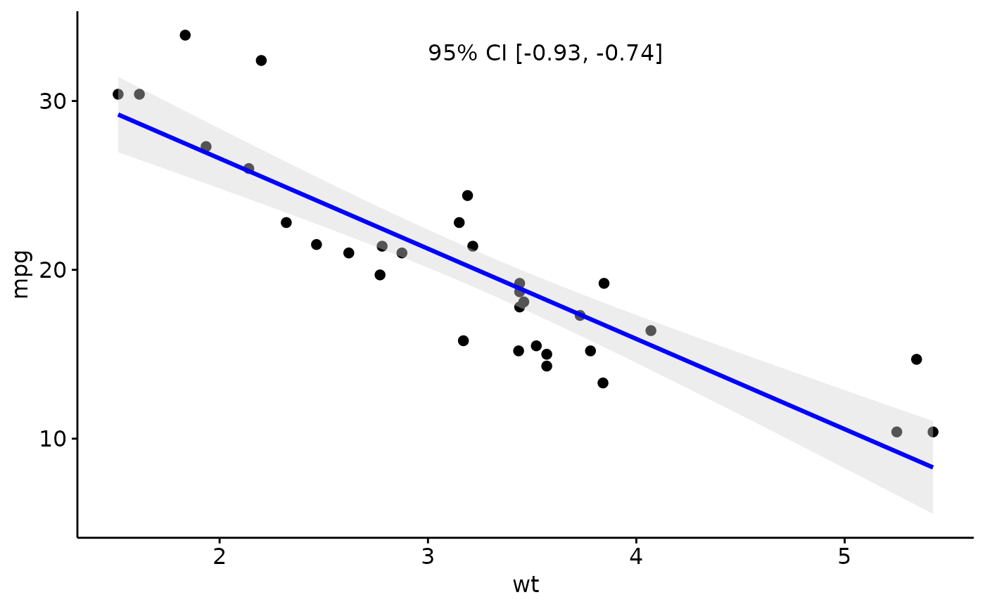
 # Show the confidence interval of the correlation coefficient (Pearson)
sp + stat_cor(aes(label = after_stat(conf.int.label)), label.x = 3)
# Show the confidence interval of the correlation coefficient (Pearson)
sp + stat_cor(aes(label = after_stat(conf.int.label)), label.x = 3)
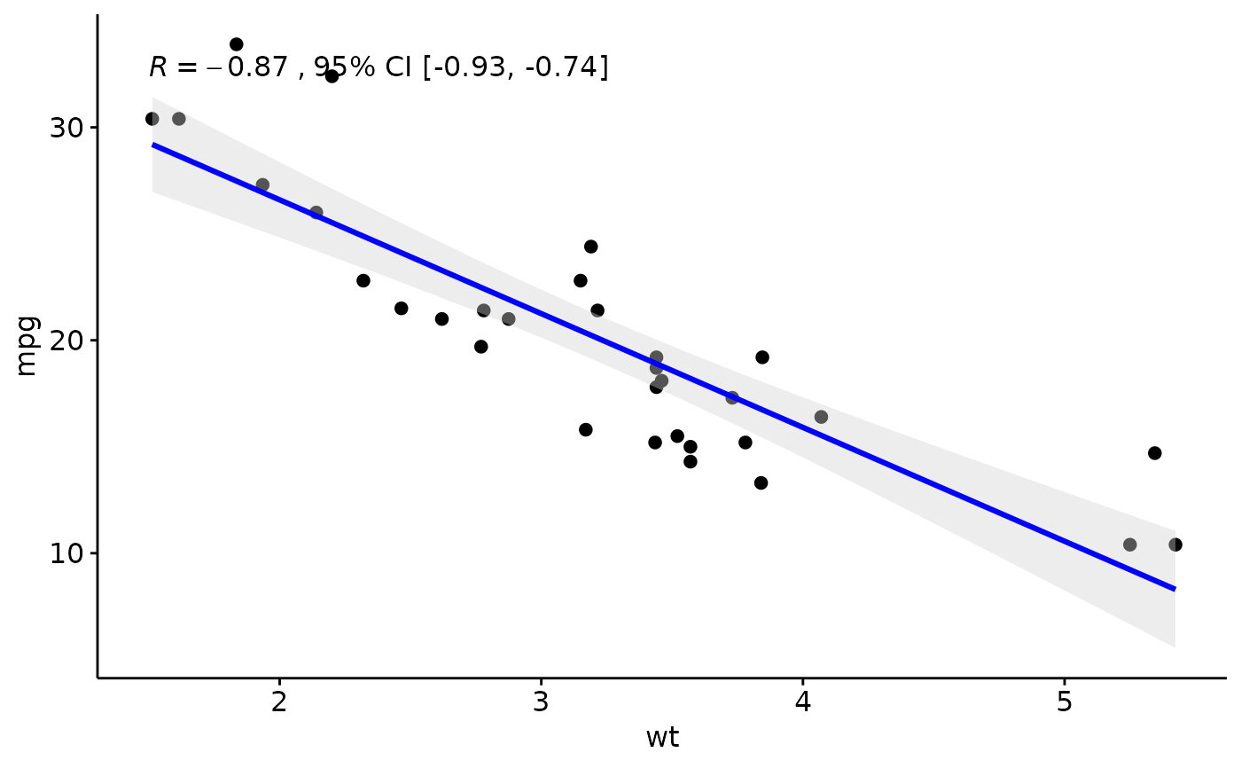
 # Correlation coefficient with its confidence interval
sp + stat_cor(
aes(label = paste(after_stat(r.label), after_stat(conf.int.label), sep = "~`,`~")),
label.x = 1.5
)
# Correlation coefficient with its confidence interval
sp + stat_cor(
aes(label = paste(after_stat(r.label), after_stat(conf.int.label), sep = "~`,`~")),
label.x = 1.5
)
 # Color by groups and facet
# ::::::::::::::::::::::::::::::::::::::::::::::::::::
sp <- ggscatter(df,
x = "wt", y = "mpg",
color = "cyl", palette = "jco",
add = "reg.line", conf.int = TRUE
)
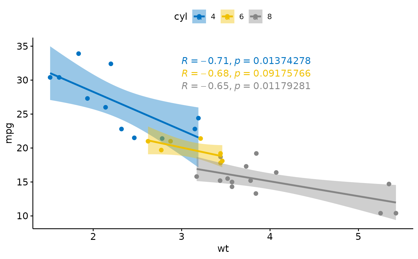
sp + stat_cor(aes(color = cyl), label.x = 3)
# Color by groups and facet
# ::::::::::::::::::::::::::::::::::::::::::::::::::::
sp <- ggscatter(df,
x = "wt", y = "mpg",
color = "cyl", palette = "jco",
add = "reg.line", conf.int = TRUE
)
sp + stat_cor(aes(color = cyl), label.x = 3)