Plot model coefficients with `ggcoef

library(ggstats)

The purpose of ggcoef_model() is to quickly plot the coefficients of a model. It is an updated and improved version of GGally::ggcoef() based on broom.helpers::tidy_plus_plus(). For displaying a nicely formatted table of the same models, look at gtsummary::tbl_regression().

Quick coefficients plot

To work automatically, this function requires the broom.helpers. Simply call ggcoef_model() with a model object. It could be the result of stats::lm, stats::glm or any other model covered by broom.helpers.

data(tips, package = "reshape")
mod_simple <- lm(tip ~ day + time + total_bill, data = tips)
ggcoef_model(mod_simple)
#> `height` was translated to `width`.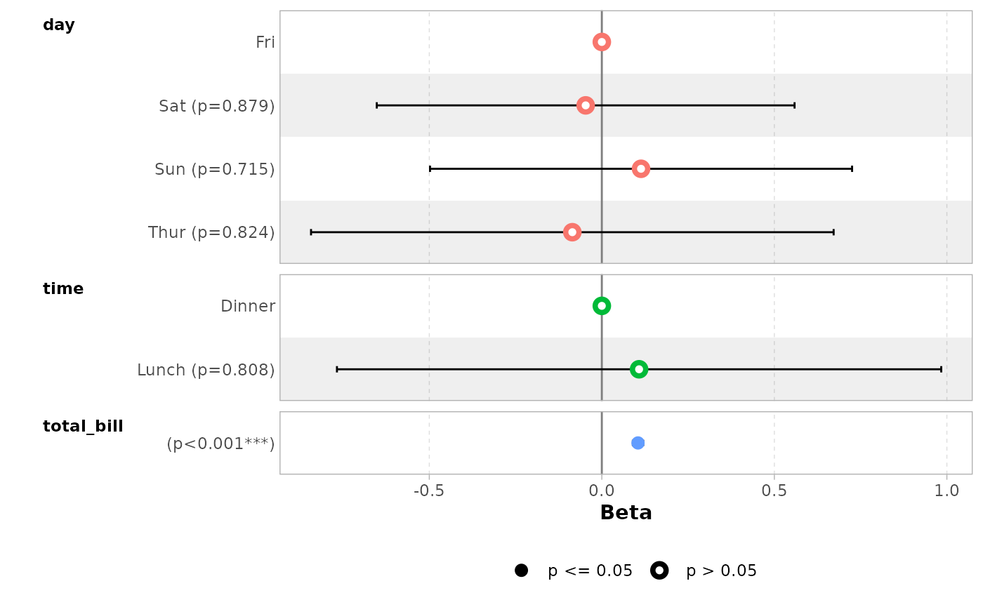

In the case of a logistic regression (or any other model for which coefficients are usually exponentiated), simply indicated exponentiate = TRUE. Note that a logarithmic scale will be used for the x-axis.

d_titanic <- as.data.frame(Titanic)
d_titanic$Survived <- factor(d_titanic$Survived, c("No", "Yes"))
mod_titanic <- glm(
  Survived ~ Sex * Age + Class,
  weights = Freq,
  data = d_titanic,
  family = binomial
)
ggcoef_model(mod_titanic, exponentiate = TRUE)
#> `height` was translated to `width`.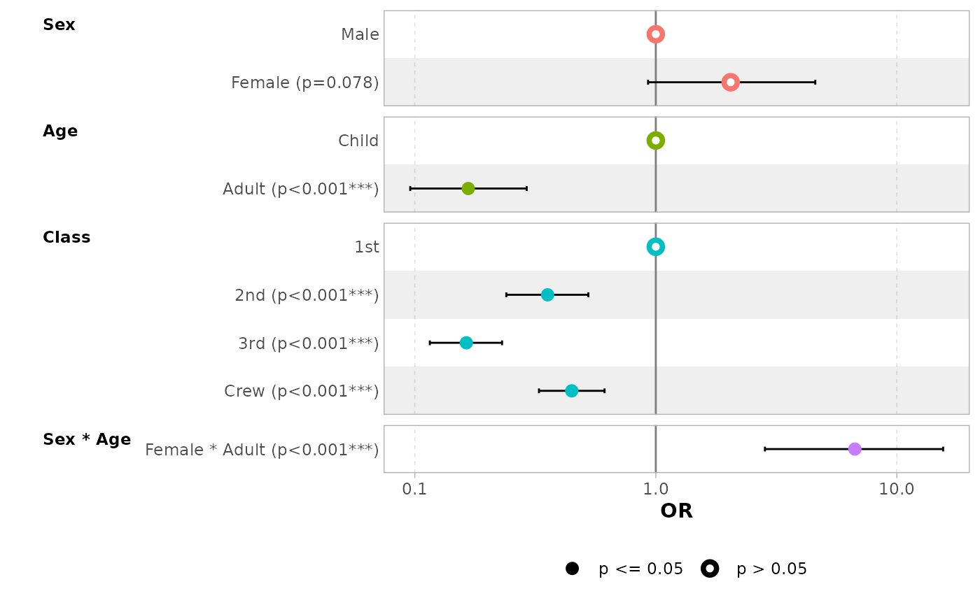

Customizing the plot

Variable labels

You can use the labelled package to define variable labels. They will be automatically used by ggcoef_model(). Note that variable labels should be defined before computing the model.

library(labelled)
tips_labelled <- tips |>
  set_variable_labels(
    day = "Day of the week",
    time = "Lunch or Dinner",
    total_bill = "Bill's total"
  )
mod_labelled <- lm(tip ~ day + time + total_bill, data = tips_labelled)
ggcoef_model(mod_labelled)
#> `height` was translated to `width`.

You can also define custom variable labels directly by passing a named vector to the variable_labels option.

ggcoef_model(
  mod_simple,
  variable_labels = c(
    day = "Week day",
    time = "Time (lunch or dinner ?)",
    total_bill = "Total of the bill"
  )
)
#> `height` was translated to `width`.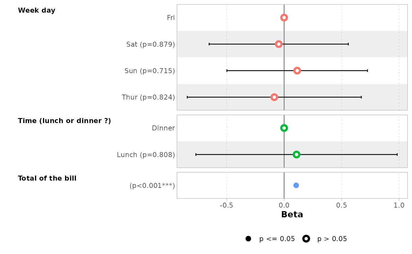

If variable labels are to long, you can pass ggplot2::label_wrap_gen() or any other labeller function to facet_labeller.

ggcoef_model(
  mod_simple,
  variable_labels = c(
    day = "Week day",
    time = "Time (lunch or dinner ?)",
    total_bill = "Total of the bill"
  ),
  facet_labeller = ggplot2::label_wrap_gen(10)
)
#> `height` was translated to `width`.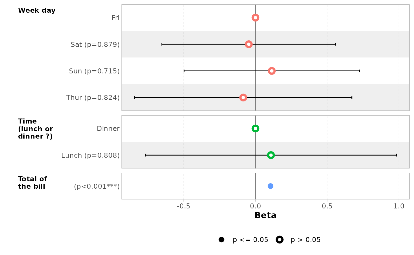

Use facet_row = NULL to hide variable names.

ggcoef_model(mod_simple, facet_row = NULL, colour_guide = TRUE)
#> `height` was translated to `width`.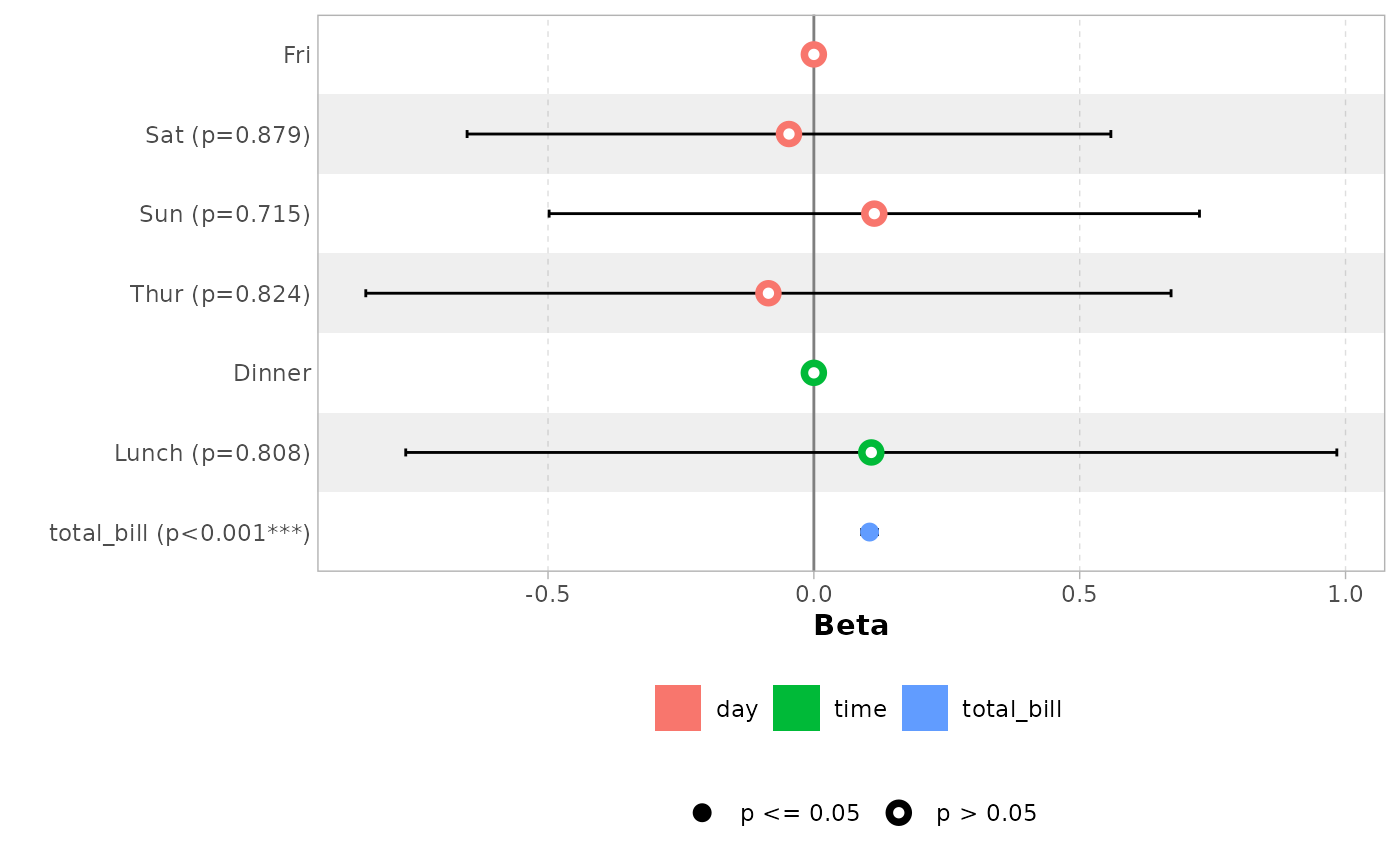

Term labels

Several options allows you to customize term labels.

ggcoef_model(mod_titanic, exponentiate = TRUE)
#> `height` was translated to `width`.

ggcoef_model(
  mod_titanic,
  exponentiate = TRUE,
  show_p_values = FALSE,
  signif_stars = FALSE,
  add_reference_rows = FALSE,
  categorical_terms_pattern = "{level} (ref: {reference_level})",
  interaction_sep = " x "
) +
  ggplot2::scale_y_discrete(labels = scales::label_wrap(15))
#> Scale for y is already present.
#> Adding another scale for y, which will replace the existing scale.
#> `height` was translated to `width`.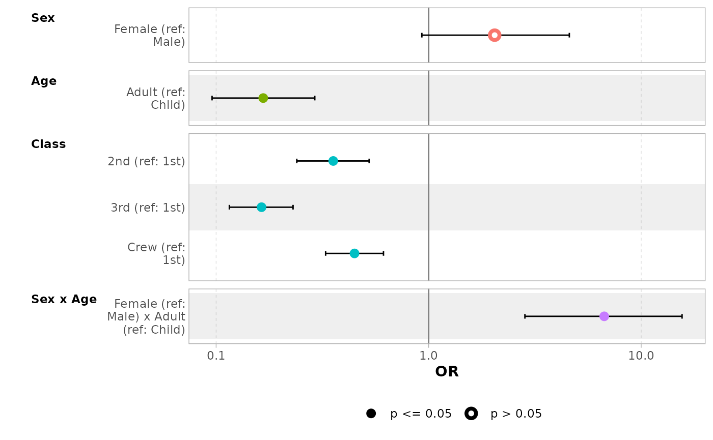

By default, for categorical variables using treatment and sum contrasts, reference rows will be added and displayed on the graph.

mod_titanic2 <- glm(
  Survived ~ Sex * Age + Class,
  weights = Freq,
  data = d_titanic,
  family = binomial,
  contrasts = list(Sex = contr.sum, Class = contr.treatment(4, base = 3))
)
ggcoef_model(mod_titanic2, exponentiate = TRUE)
#> `height` was translated to `width`.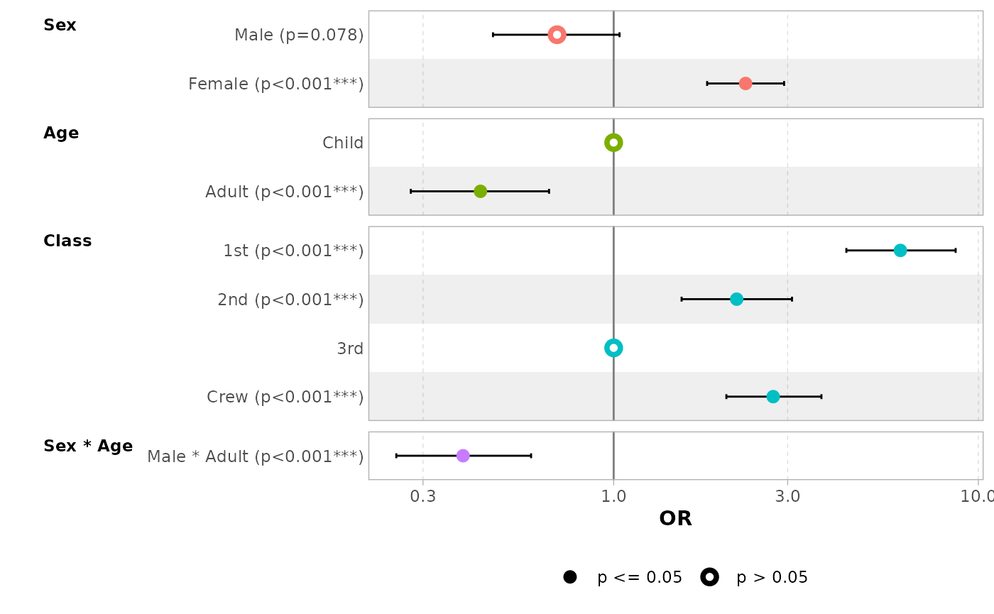

Continuous variables with polynomial terms defined with stats::poly() are also properly managed.

mod_poly <- lm(Sepal.Length ~ poly(Petal.Width, 3) + Petal.Length, data = iris)
ggcoef_model(mod_poly)
#> `height` was translated to `width`.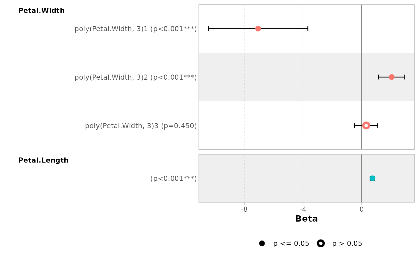

Use no_reference_row to indicate which variables should not have a reference row added.

ggcoef_model(
  mod_titanic2,
  exponentiate = TRUE,
  no_reference_row = "Sex"
)
#> `height` was translated to `width`.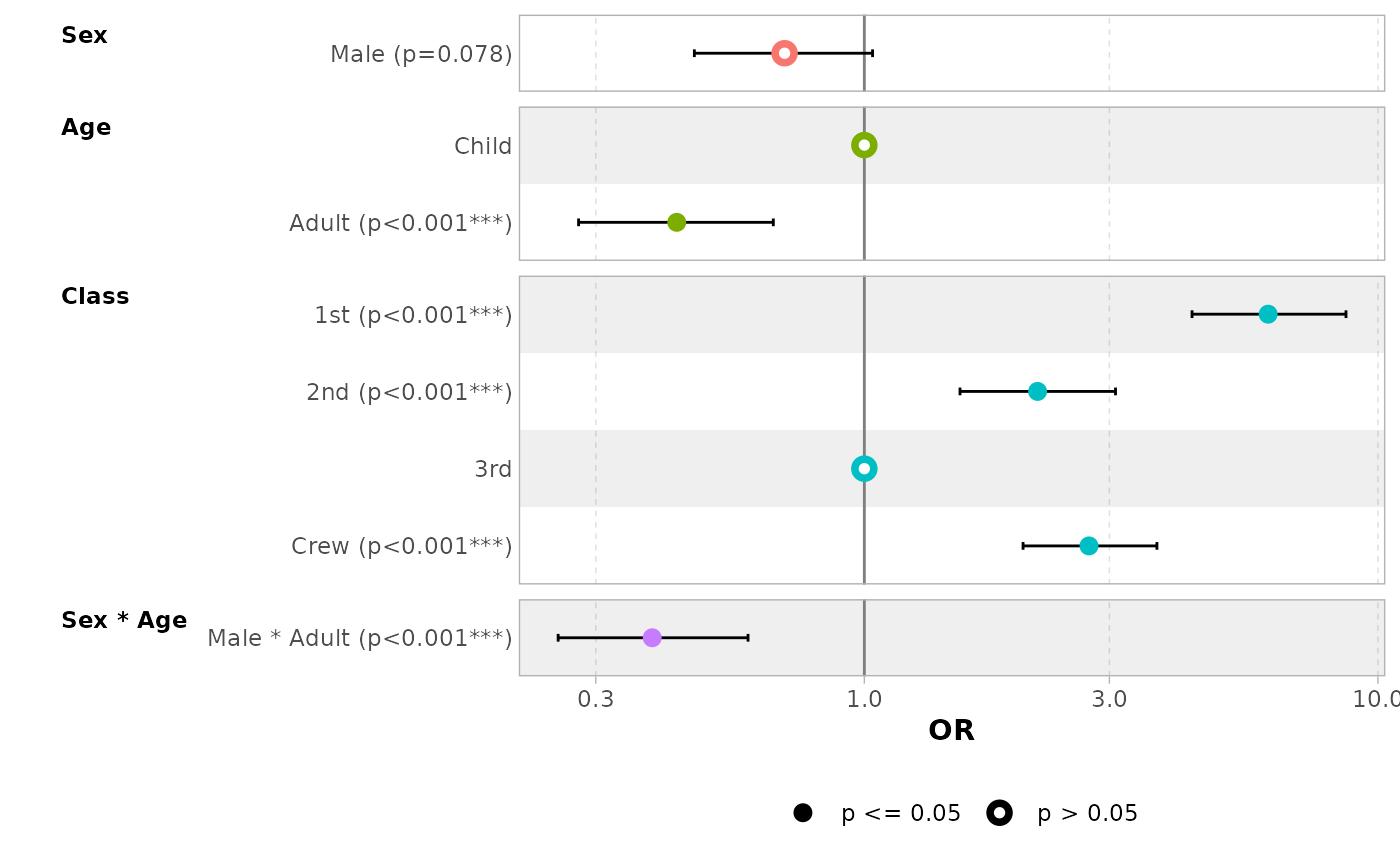

ggcoef_model(
  mod_titanic2,
  exponentiate = TRUE,
  no_reference_row = broom.helpers::all_dichotomous()
)
#> `height` was translated to `width`.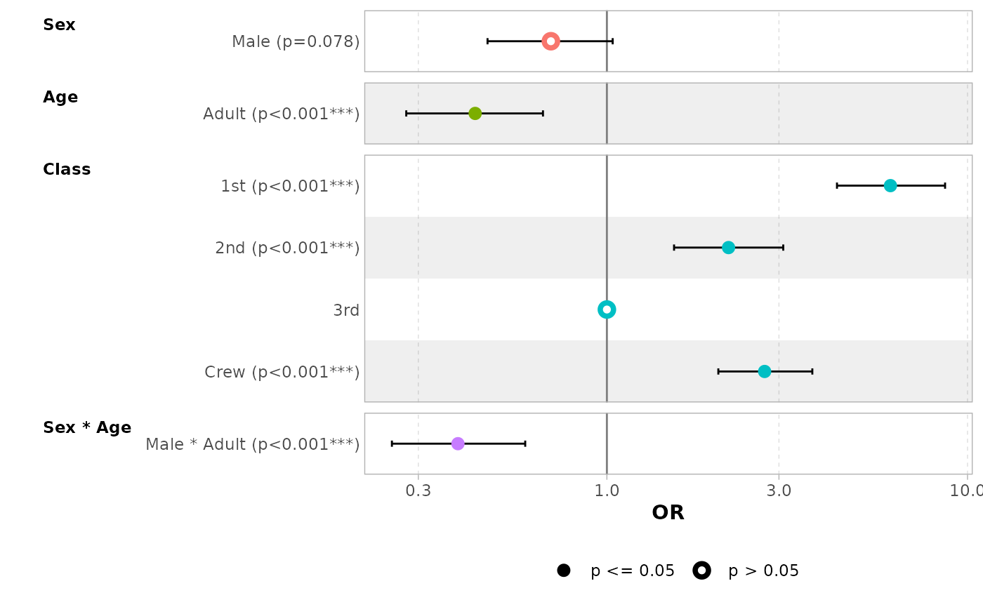

ggcoef_model(
  mod_titanic2,
  exponentiate = TRUE,
  no_reference_row = broom.helpers::all_categorical(),
  categorical_terms_pattern = "{level}/{reference_level}"
)
#> `height` was translated to `width`.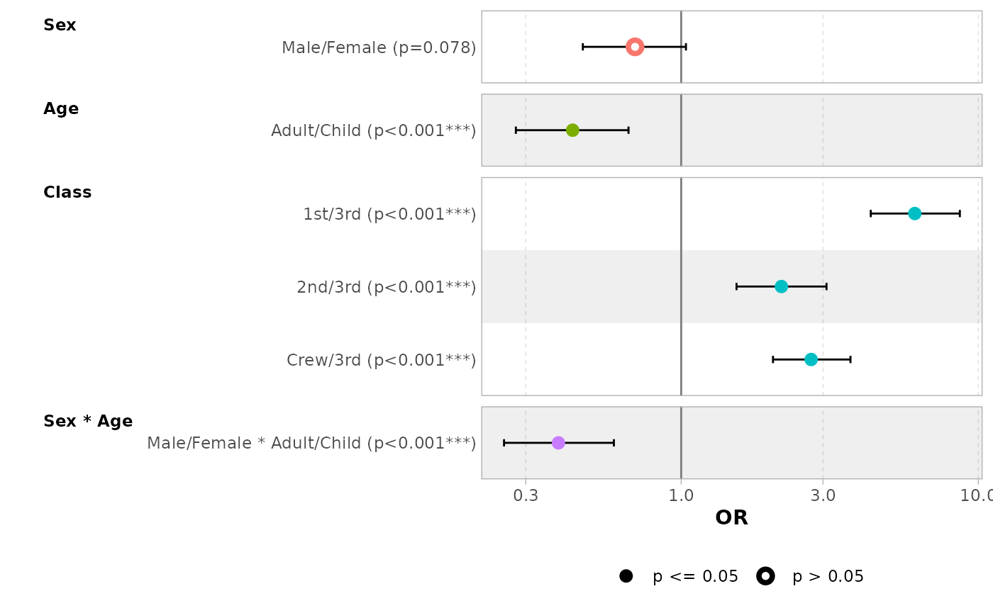

Elements to display

Use intercept = TRUE to display intercepts.

ggcoef_model(mod_simple, intercept = TRUE)
#> `height` was translated to `width`.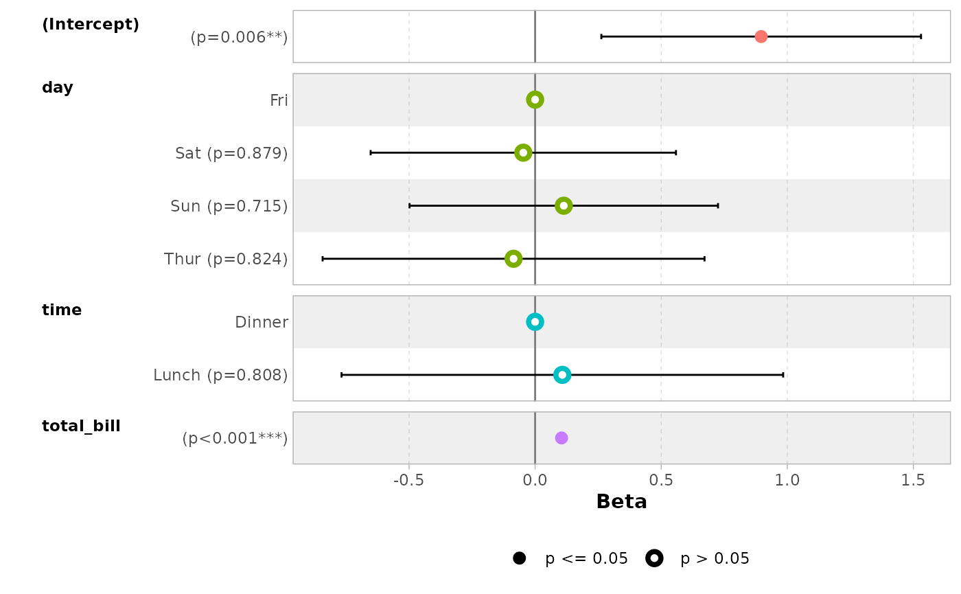

You can remove confidence intervals with conf.int = FALSE.

ggcoef_model(mod_simple, conf.int = FALSE)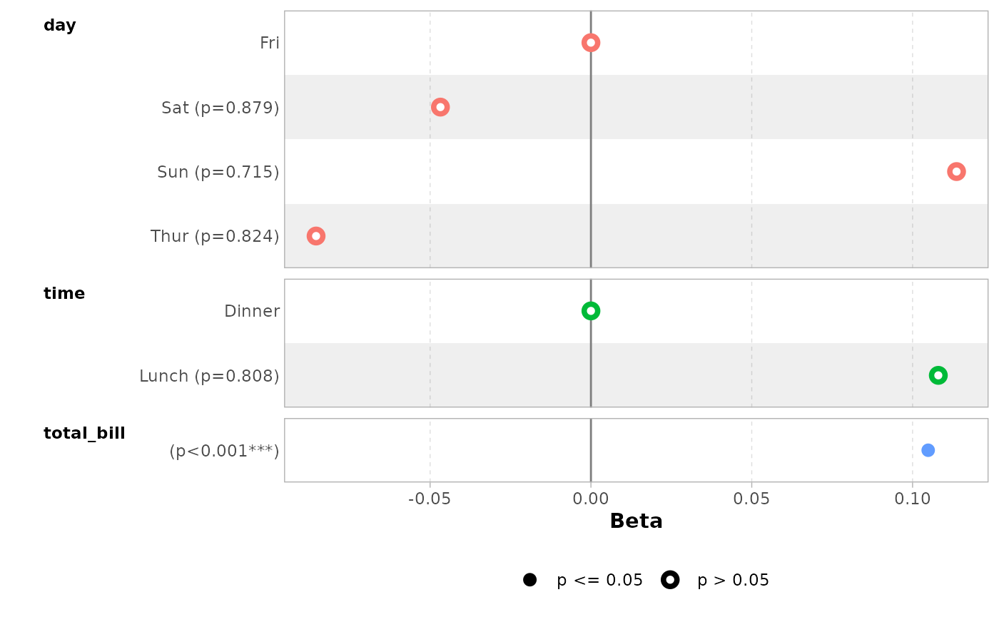

By default, significant terms (i.e. with a p-value below 5%) are highlighted using two types of dots. You can control the level of significance with significance or remove it with significance = NULL.

ggcoef_model(mod_simple, significance = NULL)
#> `height` was translated to `width`.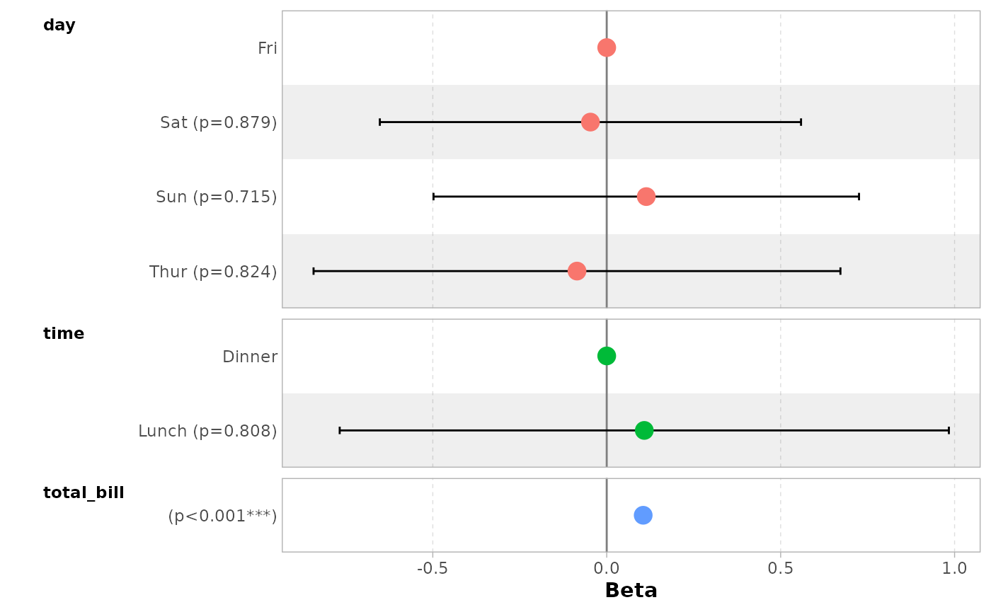

By default, dots are colored by variable. You can deactivate this behavior with colour = NULL.

ggcoef_model(mod_simple, colour = NULL)
#> `height` was translated to `width`.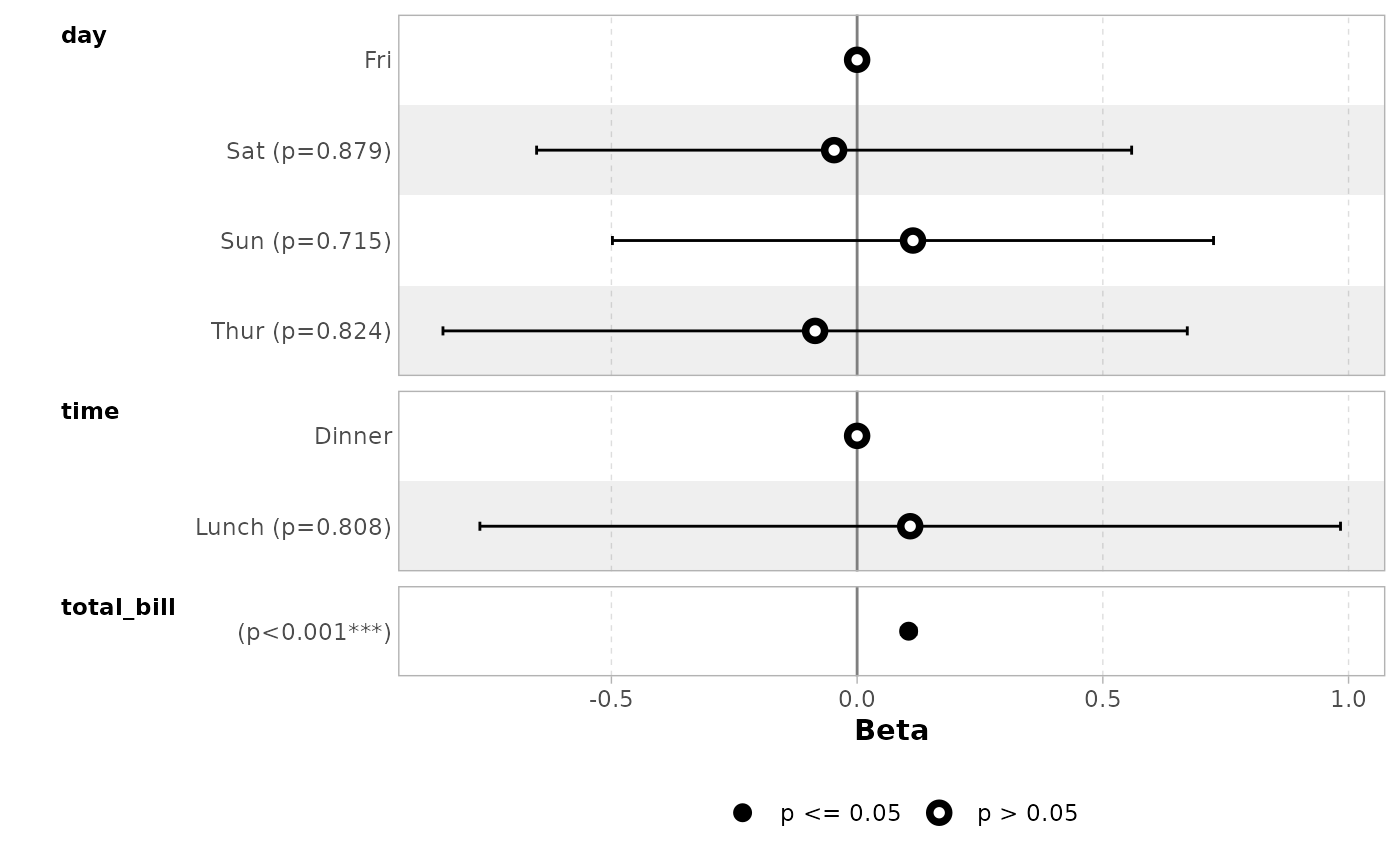

You can display only a subset of terms with include.

ggcoef_model(mod_simple, include = c("time", "total_bill"))
#> `height` was translated to `width`.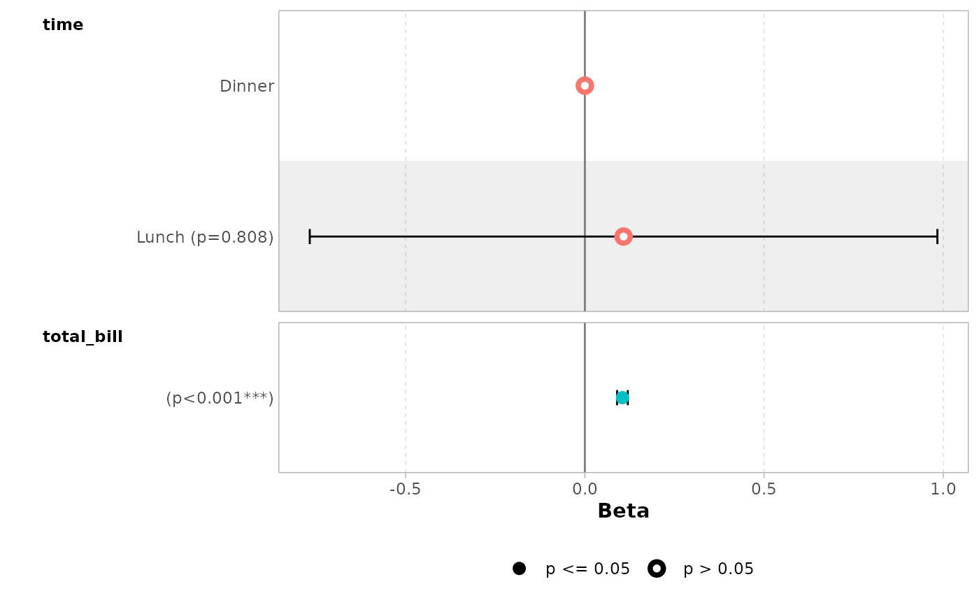

It is possible to use tidyselect helpers.

ggcoef_model(mod_simple, include = dplyr::starts_with("t"))
#> `height` was translated to `width`.

You can remove stripped rows with stripped_rows = FALSE.

ggcoef_model(mod_simple, stripped_rows = FALSE)
#> `height` was translated to `width`.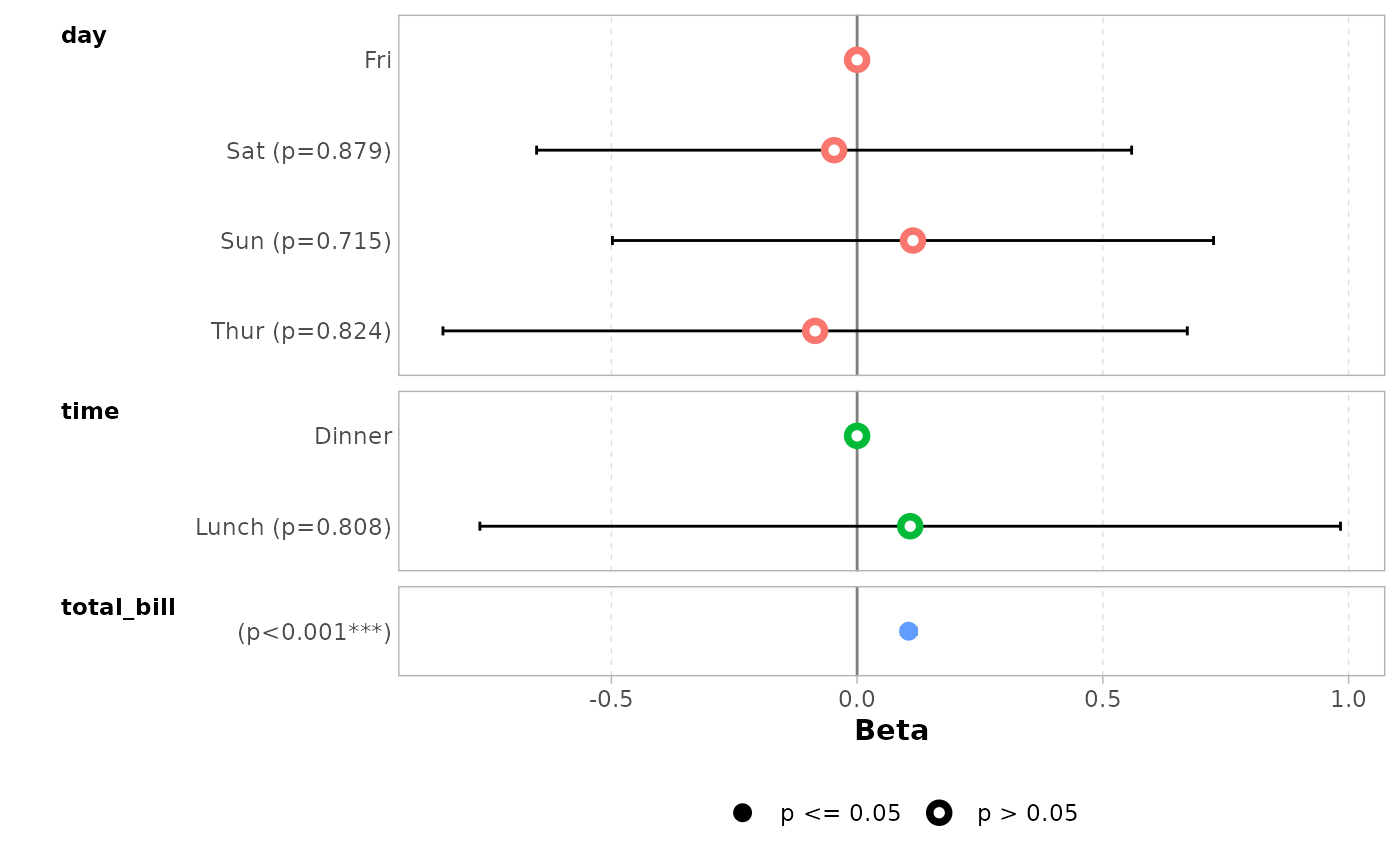

Do not hesitate to consult the help file of ggcoef_model() to see all available options.

ggplot2 elements

The plot returned by ggcoef_model() is a classic ggplot2 plot. You can therefore apply ggplot2 functions to it.

ggcoef_model(mod_simple) +
  ggplot2::xlab("Coefficients") +
  ggplot2::ggtitle("Custom title") +
  ggplot2::scale_color_brewer(palette = "Set1") +
  ggplot2::theme(legend.position = "right")
#> Scale for colour is already present.
#> Adding another scale for colour, which will replace the existing scale.
#> `height` was translated to `width`.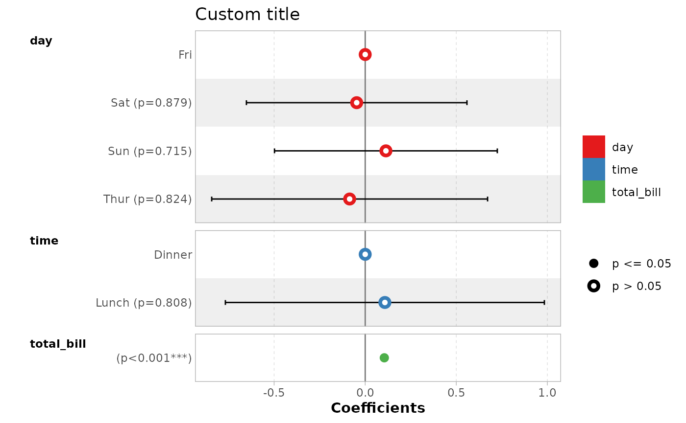

Forest plot with a coefficient table

ggcoef_table() is a variant of ggcoef_model() displaying a coefficient table on the right of the forest plot.

ggcoef_table(mod_simple)
#> `height` was translated to `width`.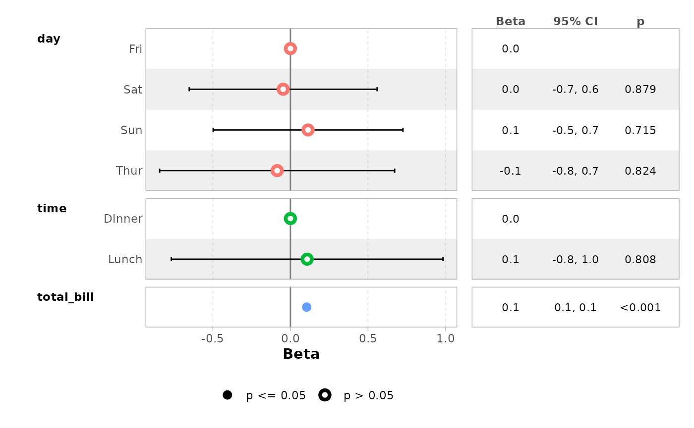

ggcoef_table(mod_titanic, exponentiate = TRUE)
#> `height` was translated to `width`.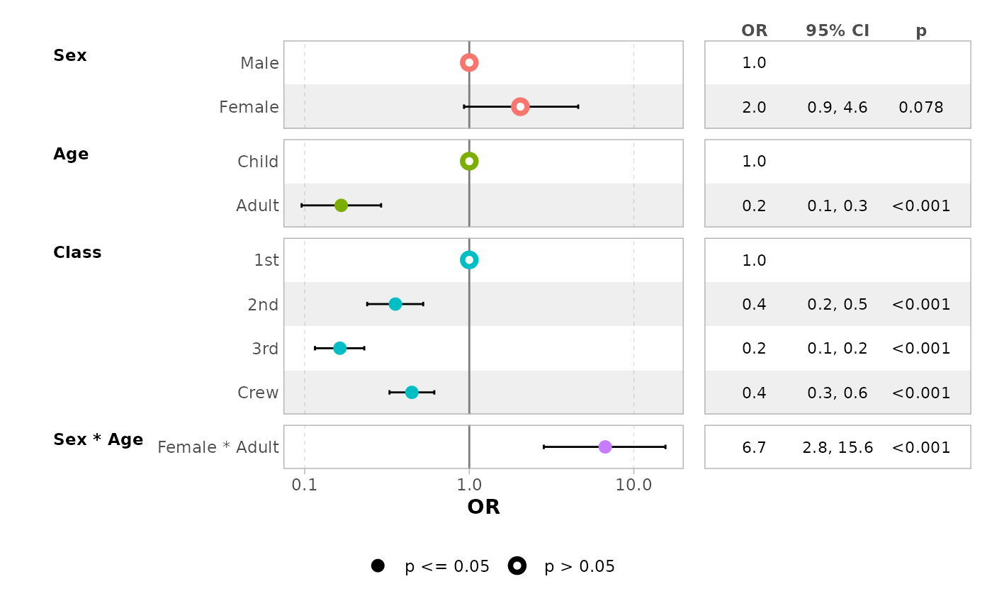

You can easily customize the columns to be displayed.

ggcoef_table(
  mod_simple,
  table_stat = c("label", "estimate", "std.error", "ci"),
  ci_pattern = "{conf.low} to {conf.high}",
  table_stat_label = list(
    estimate = scales::label_number(accuracy = .001),
    conf.low = scales::label_number(accuracy = .01),
    conf.high = scales::label_number(accuracy = .01),
    std.error = scales::label_number(accuracy = .001),
    label = toupper
  ),
  table_header = c("Term", "Coef.", "SE", "CI"),
  table_witdhs = c(2, 3)
)
#> `height` was translated to `width`.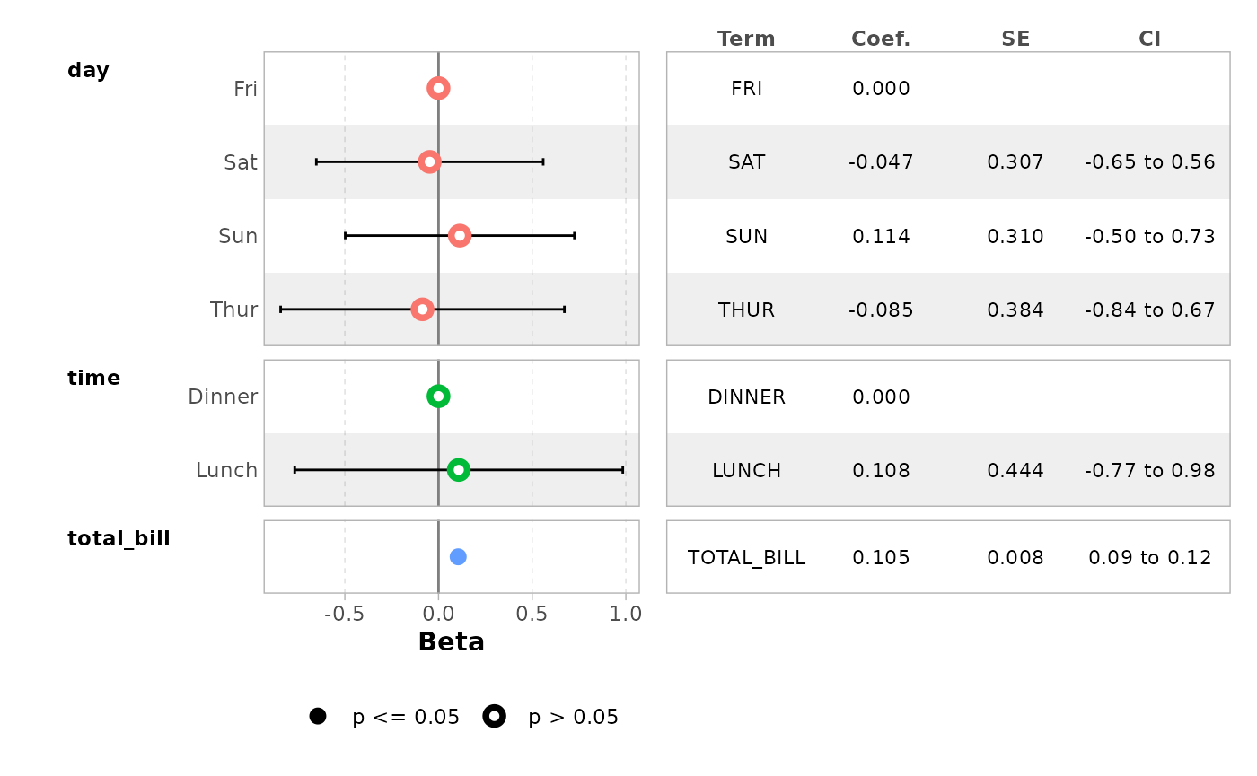

Multinomial models

For multinomial models, simply use ggcoef_multinom(). Three types of visualizations are available: "dodged", "faceted" and "table".

library(nnet)
hec <- as.data.frame(HairEyeColor)
mod <- multinom(
  Hair ~ Eye + Sex,
  data = hec,
  weights = hec$Freq
)
#> # weights:  24 (15 variable)
#> initial  value 820.686262 
#> iter  10 value 669.061500
#> iter  20 value 658.888977
#> final  value 658.885327 
#> converged
ggcoef_multinom(
  mod,
  exponentiate = TRUE
)
#> `height` was translated to `width`.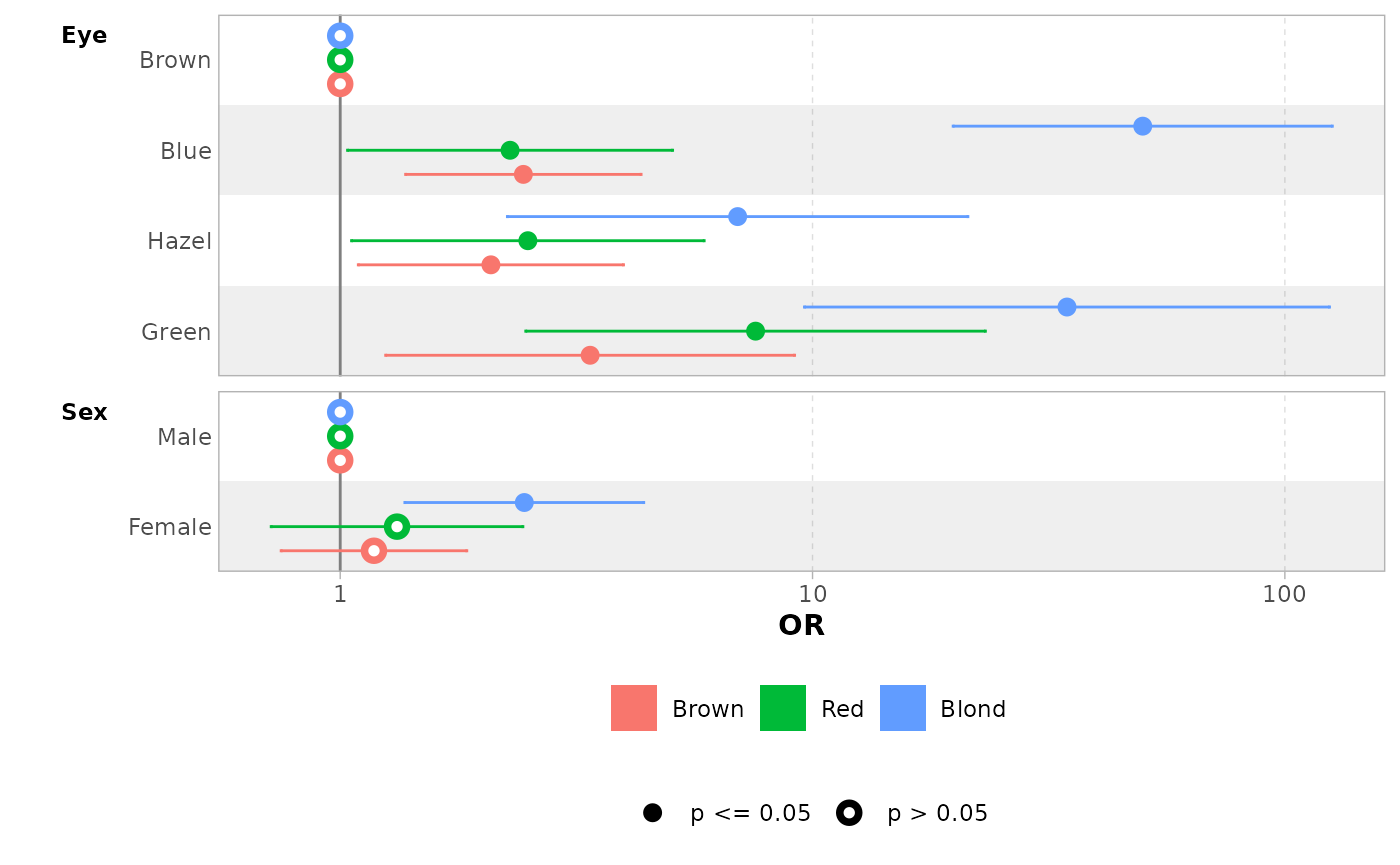

ggcoef_multinom(
  mod,
  exponentiate = TRUE,
  type = "faceted"
)
#> `height` was translated to `width`.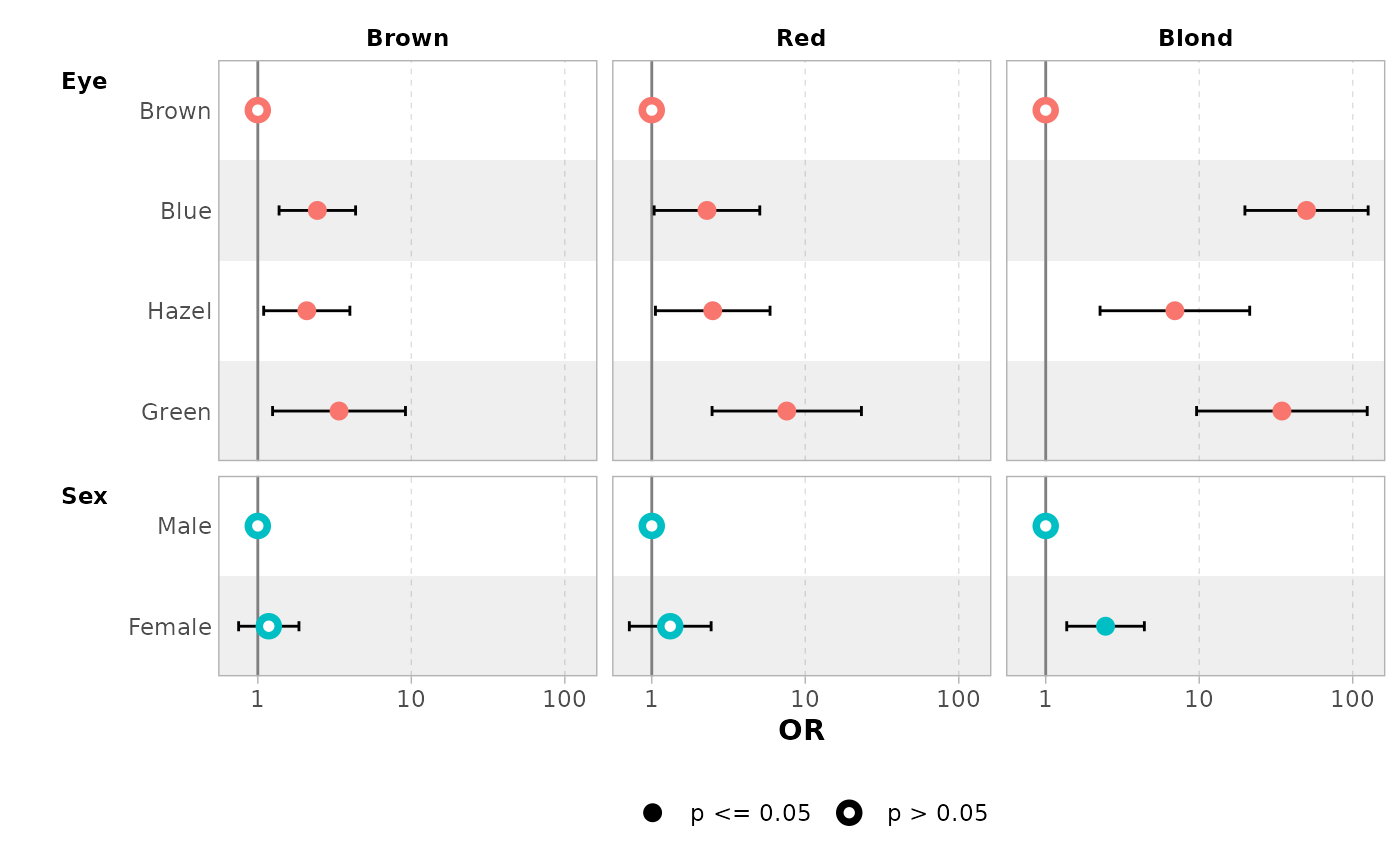

ggcoef_multinom(
  mod,
  exponentiate = TRUE,
  type = "table"
)
#> `height` was translated to `width`.
#> `height` was translated to `width`.
#> `height` was translated to `width`.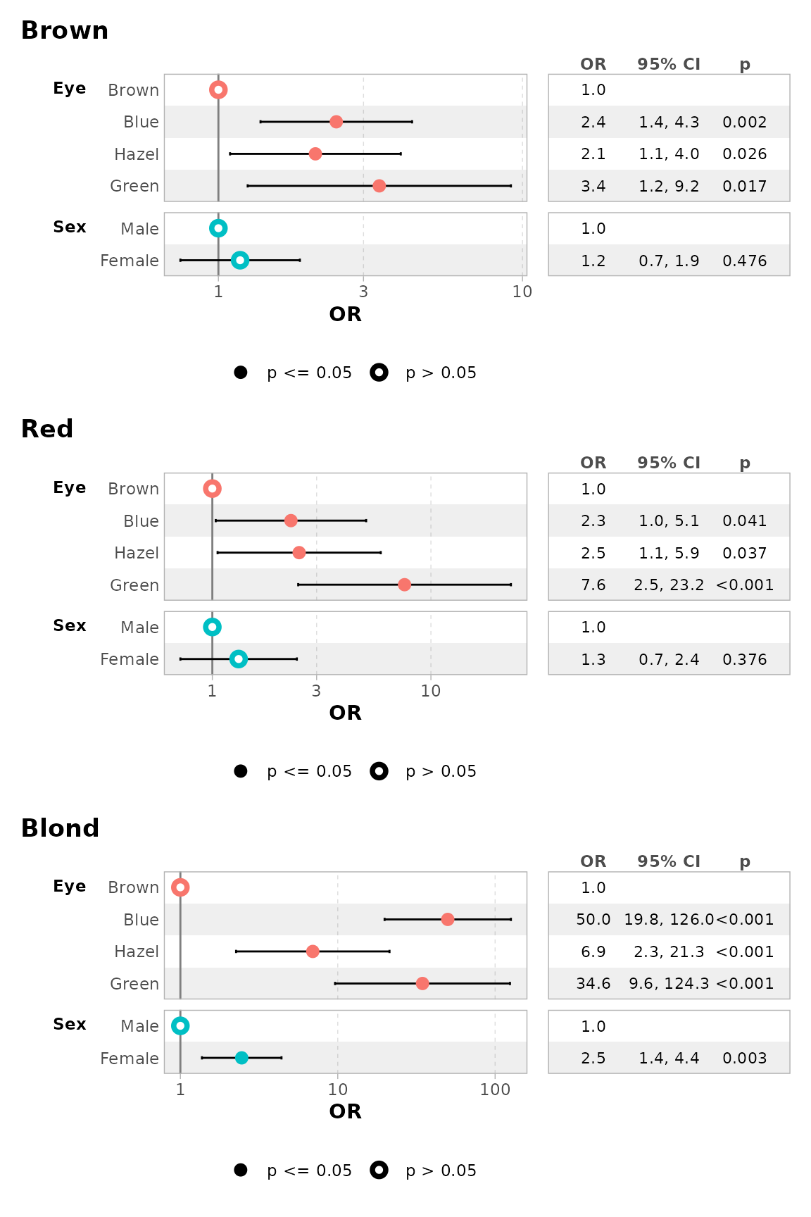

You can use y.level_label to customize the label of each level.

ggcoef_multinom(
  mod,
  type = "faceted",
  y.level_label = c("Brown" = "Brown\n(ref: Black)"),
  exponentiate = TRUE
)
#> `height` was translated to `width`.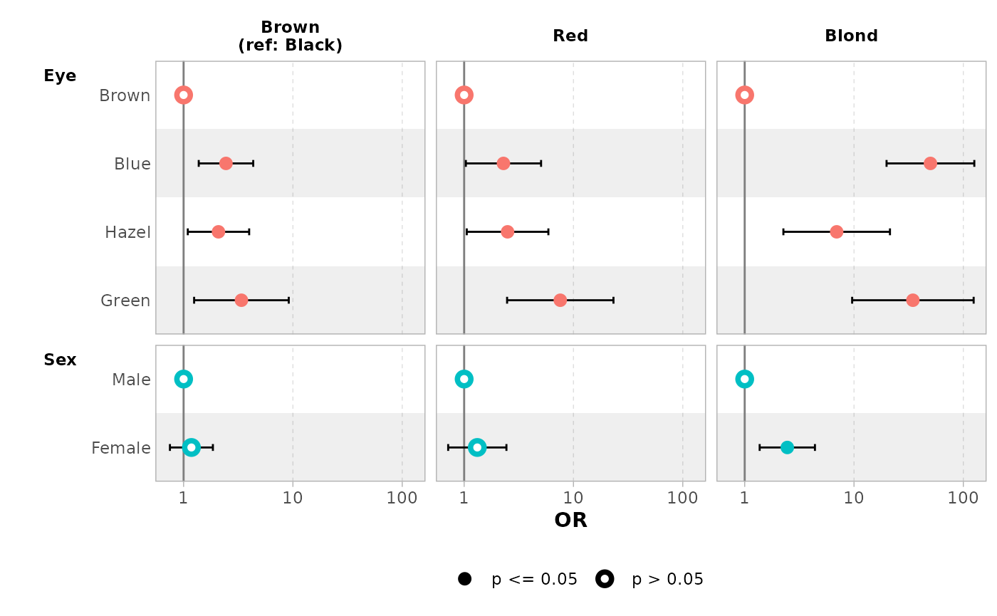

Multi-components models

Multi-components models such as zero-inflated Poisson or beta regression generate a set of terms for each of their components. You can use ggcoef_multicomponents() which is similar to ggcoef_multinom().

library(pscl)
#> Classes and Methods for R originally developed in the
#> Political Science Computational Laboratory
#> Department of Political Science
#> Stanford University (2002-2015),
#> by and under the direction of Simon Jackman.
#> hurdle and zeroinfl functions by Achim Zeileis.
data("bioChemists", package = "pscl")
mod <- zeroinfl(art ~ fem * mar | fem + mar, data = bioChemists)

ggcoef_multicomponents(mod)
#> ℹ <zeroinfl> model detected.
#> ✔ `tidy_zeroinfl()` used instead.
#> ℹ Add `tidy_fun = broom.helpers::tidy_zeroinfl` to quiet these messages.
#> `height` was translated to `width`.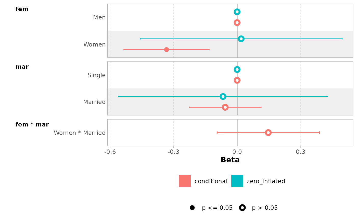

ggcoef_multicomponents(mod, type = "f")
#> ℹ <zeroinfl> model detected.
#> ✔ `tidy_zeroinfl()` used instead.
#> ℹ Add `tidy_fun = broom.helpers::tidy_zeroinfl` to quiet these messages.
#> `height` was translated to `width`.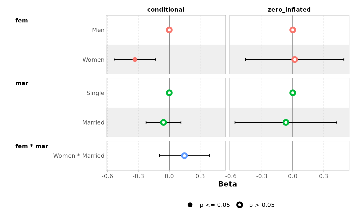

ggcoef_multicomponents(mod, type = "t")
#> ℹ <zeroinfl> model detected.
#> ✔ `tidy_zeroinfl()` used instead.
#> ℹ Add `tidy_fun = broom.helpers::tidy_zeroinfl` to quiet these messages.
#> `height` was translated to `width`.
#> `height` was translated to `width`.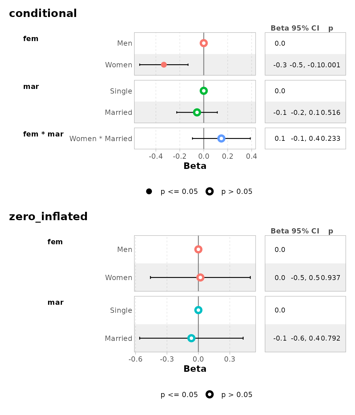

ggcoef_multicomponents(
  mod,
  type = "t",
  component_label = c(conditional = "Count", zero_inflated = "Zero-inflated")
)
#> ℹ <zeroinfl> model detected.
#> ✔ `tidy_zeroinfl()` used instead.
#> ℹ Add `tidy_fun = broom.helpers::tidy_zeroinfl` to quiet these messages.
#> `height` was translated to `width`.`height` was translated to `width`.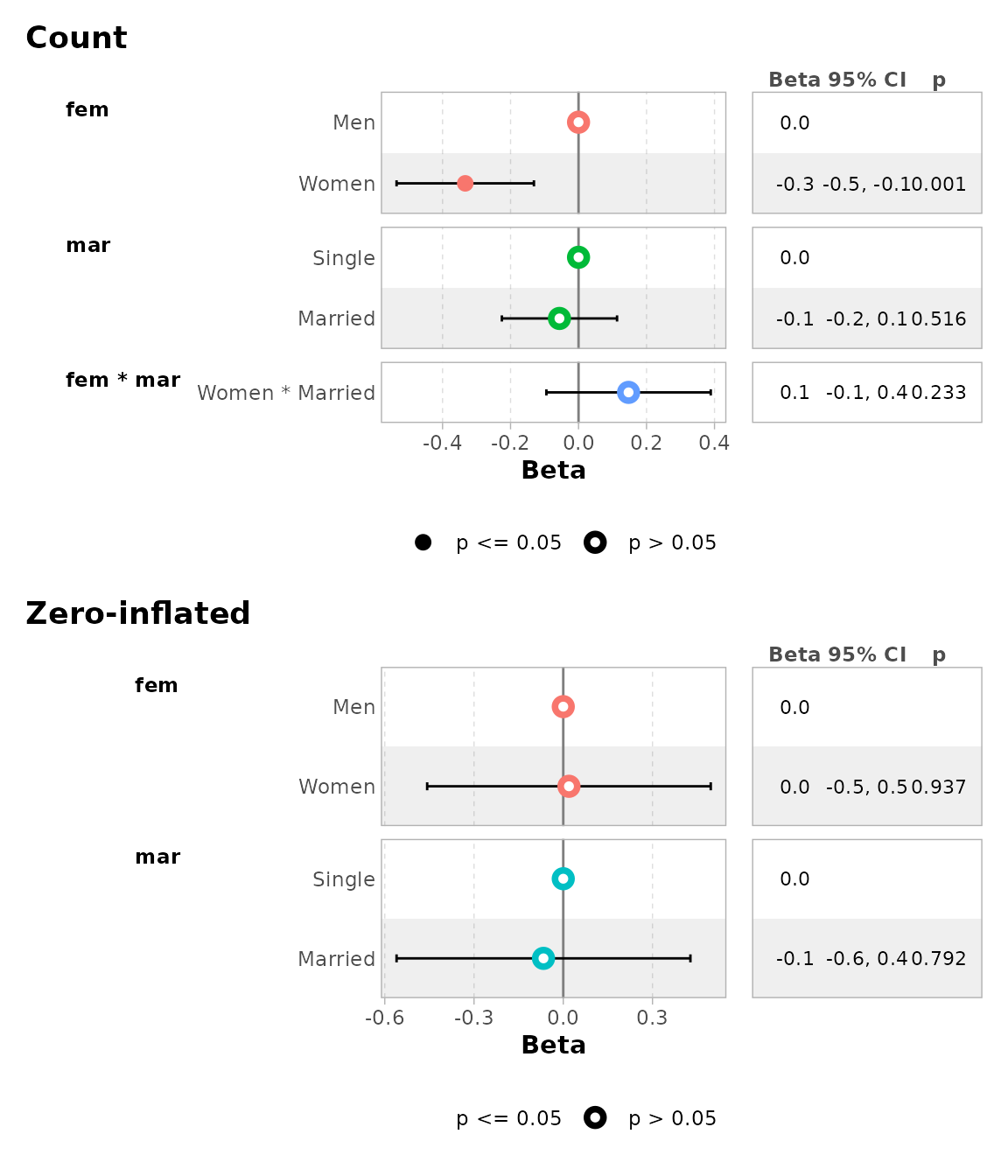

Comparing several models

You can easily compare several models with ggcoef_compare(). To be noted, ggcoef_compare() is not compatible with multinomial or multi-components models.

mod1 <- lm(Fertility ~ ., data = swiss)
mod2 <- step(mod1, trace = 0)
mod3 <- lm(Fertility ~ Agriculture + Education * Catholic, data = swiss)
models <- list(
  "Full model" = mod1,
  "Simplified model" = mod2,
  "With interaction" = mod3
)

ggcoef_compare(models)
#> `height` was translated to `width`.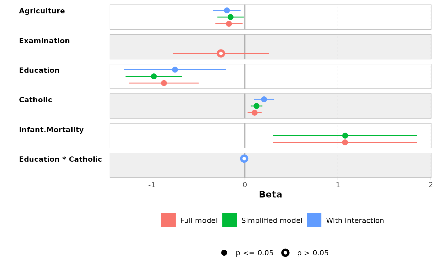

ggcoef_compare(models, type = "faceted")
#> `height` was translated to `width`.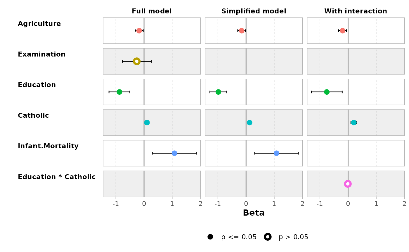

Advanced users

Advanced users could use their own dataset and pass it to ggcoef_plot(). Such dataset could be produced by ggcoef_model(), ggcoef_compare() or ggcoef_multinom() with the option return_data = TRUE or by using broom::tidy() or broom.helpers::tidy_plus_plus().

Supported models

model	notes
`betareg::betareg()`	Use `tidy_parameters()` as `tidy_fun` with `component` argument to control with coefficients to return. `broom::tidy()` does not support the `exponentiate` argument for betareg models, use `tidy_parameters()` instead.
`biglm::bigglm()`
`brms::brm()`	`broom.mixed` package required
`cmprsk::crr()`	Limited support. It is recommended to use `tidycmprsk::crr()` instead.
`fixest::feglm()`	May fail with R <= 4.0.
`fixest::femlm()`	May fail with R <= 4.0.
`fixest::feNmlm()`	May fail with R <= 4.0.
`fixest::feols()`	May fail with R <= 4.0.
`gam::gam()`
`geepack::geeglm()`
`glmmTMB::glmmTMB()`	`broom.mixed` package required
`glmtoolbox::glmgee()`
`lavaan::lavaan()`	Limited support for categorical variables
`lfe::felm()`
`lme4::glmer.nb()`	`broom.mixed` package required
`lme4::glmer()`	`broom.mixed` package required
`lme4::lmer()`	`broom.mixed` package required
`logitr::logitr()`	Requires logitr >= 0.8.0
`MASS::glm.nb()`
`MASS::polr()`
`mgcv::gam()`	Use default tidier `broom::tidy()` for smooth terms only, or `gtsummary::tidy_gam()` to include parametric terms
`mice::mira`	Limited support. If `mod` is a `mira` object, use `tidy_fun = function(x, ...) {mice::pool(x) \|> mice::tidy(...)}`
`mmrm::mmrm()`
`multgee::nomLORgee()`	Use `tidy_multgee()` as `tidy_fun`.
`multgee::ordLORgee()`	Use `tidy_multgee()` as `tidy_fun`.
`nnet::multinom()`
`ordinal::clm()`	Limited support for models with nominal predictors.
`ordinal::clmm()`	Limited support for models with nominal predictors.
`parsnip::model_fit`	Supported as long as the type of model and the engine is supported.
`plm::plm()`
`pscl::hurdle()`	Use `tidy_zeroinfl()` as `tidy_fun`.
`pscl::zeroinfl()`	Use `tidy_zeroinfl()` as `tidy_fun`.
`quantreg::rq()`	If several quantiles are estimated, use `tidy_with_broom_or_parameters()` tidier, the default tidier used by `tidy_plus_plus()`.
`rstanarm::stan_glm()`	`broom.mixed` package required
`stats::aov()`	Reference rows are not relevant for such models.
`stats::glm()`
`stats::lm()`
`stats::nls()`	Limited support
`survey::svycoxph()`
`survey::svyglm()`
`survey::svyolr()`
`survival::cch()`	Experimental support.
`survival::clogit()`
`survival::coxph()`
`survival::survreg()`
`svyVGAM::svy_vglm()`	Experimental support. It is recommended to use `tidy_svy_vglm()` as `tidy_fun`.
`tidycmprsk::crr()`
`VGAM::vgam()`	Experimental support. It is recommended to use `tidy_vgam()` as `tidy_fun`.
`VGAM::vglm()`	Experimental support. It is recommended to use `tidy_vgam()` as `tidy_fun`.

Note: this list of models has been tested. broom.helpers, and therefore ggcoef_model(), may or may not work properly or partially with other types of models.

Plot model coefficients with `ggcoef_model()`

Joseph Larmarange

Quick coefficients plot

Customizing the plot

Variable labels

Term labels

Elements to display

ggplot2 elements

Forest plot with a coefficient table

Multinomial models

Multi-components models

Comparing several models

Advanced users

Supported models

Plot model coefficients with ggcoef_model()

Joseph Larmarange

Quick coefficients plot

Customizing the plot

Variable labels

Term labels

Elements to display

ggplot2 elements

Forest plot with a coefficient table

Multinomial models

Multi-components models

Comparing several models

Advanced users

Supported models

Plot model coefficients with `ggcoef_model()`