Draw a line with a label, by default its equation
panel.lmlineq.RdThis is an extension of the panel functions panel.abline and
panel.lmline to also draw a label on the line. The
default label is the line equation, and optionally the R squared value
of its fit to the data points.
panel.ablineq(a = NULL, b = 0,
              h = NULL, v = NULL,
              reg = NULL, coef = NULL,
              pos = if (rotate) 1 else NULL,
              offset = 0.5, adj = NULL,
              at = 0.5, x, y,
              rotate = FALSE, srt = 0,
              label = NULL,
              varNames = alist(y = y, x = x),
              varStyle = "italic",
              fontfamily = "serif",
              digits = 3,
              r.squared = FALSE, sep = ", ", sep.end = "",
              col, col.text, col.line,
              ..., reference = FALSE)

panel.lmlineq(x, y, ...)
Arguments
- a, b, h, v, reg, coef
specification of the line. The simplest usage is to give
aandbto describe the line y = a + b x. Horizontal or vertical lines can be specified as argumentshorv, respectively. The first argument (a) can also be a model object produced bylm. Seepanel.ablinefor more details.- pos, offset
passed on to
panel.text. Forpos: 1 = below, 2 = left, 3 = above, 4 = right, and theoffset(in character widths) is applied.- adj
passed on to
panel.text. c(0,0) = above right, c(1,0) = above left, c(0,1) = below right, c(1,1) = below left; offset does not apply when usingadj.- fontfamily
passed on to
panel.text.- at
position of the equation as a fractional distance along the line. This should be in the range 0 to 1. When a vertical line is drawn, this gives the vertical position of the equation.
- x, y
position of the equation in native units. If given, this over-rides
at. Forpanel.lmlineqthis is the data, passed on aslm(y ~ x).- rotate, srt
set
rotate = TRUEto align the equation with the line. This will over-ridesrt, which otherwise gives the rotation angle. Note that the calculated angle depends on the current device size; this will be wrong if you change the device aspect ratio after plotting.- label
the text to draw along with the line. If specified, this will be used instead of an equation.
- varNames
names to display for
xand/ory. This should be a list likelist(y = "Q", x = "X")or, for mathematical symbols,alist(y = (alpha + beta), x = sqrt(x[t])).- varStyle
the name of a
plotmathfunction to wrap around the equation expression, orNULL. E.g."bolditalic","displaystyle".- digits
number of decimal places to show for coefficients in equation.
- r.squared
the \(R^2\) statistic to display along with the equation of a line. This can be given directly as a number, or
TRUE, in which case the function expects a model object (typicallylm) and extracts the \(R^2\) statistic from it.- sep, sep.end
The \(R^2\) (
r.squared) value is separated from the equation by the stringsep, and alsosep.endis added to the end. For example:panel.ablineq(lm(y ~ x), r.squared = TRUE, sep = " (", sep.end = ")").- ..., col, col.text, col.line
passed on to
panel.ablineandpanel.text. Note thatcolapplies to both text and line;col.textapplies to the equation only, andcol.lineapplies to line only.- reference
whether to draw the line in a "reference line" style, like that used for grid lines.
Details
The equation is constructed as an expression using plotmath.
See also
Examples
set.seed(0)
xsim <- rnorm(50, mean = 3)
ysim <- (0 + 2 * xsim) * (1 + rnorm(50, sd = 0.3))
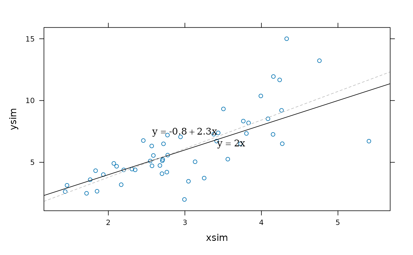
## basic use as a panel function
xyplot(ysim ~ xsim, panel = function(x, y, ...) {
panel.xyplot(x, y, ...)
panel.ablineq(a = 0, b = 2, adj = c(0,1))
panel.lmlineq(x, y, adj = c(1,0), lty = 2,
col.line = "grey", digits = 1)
})
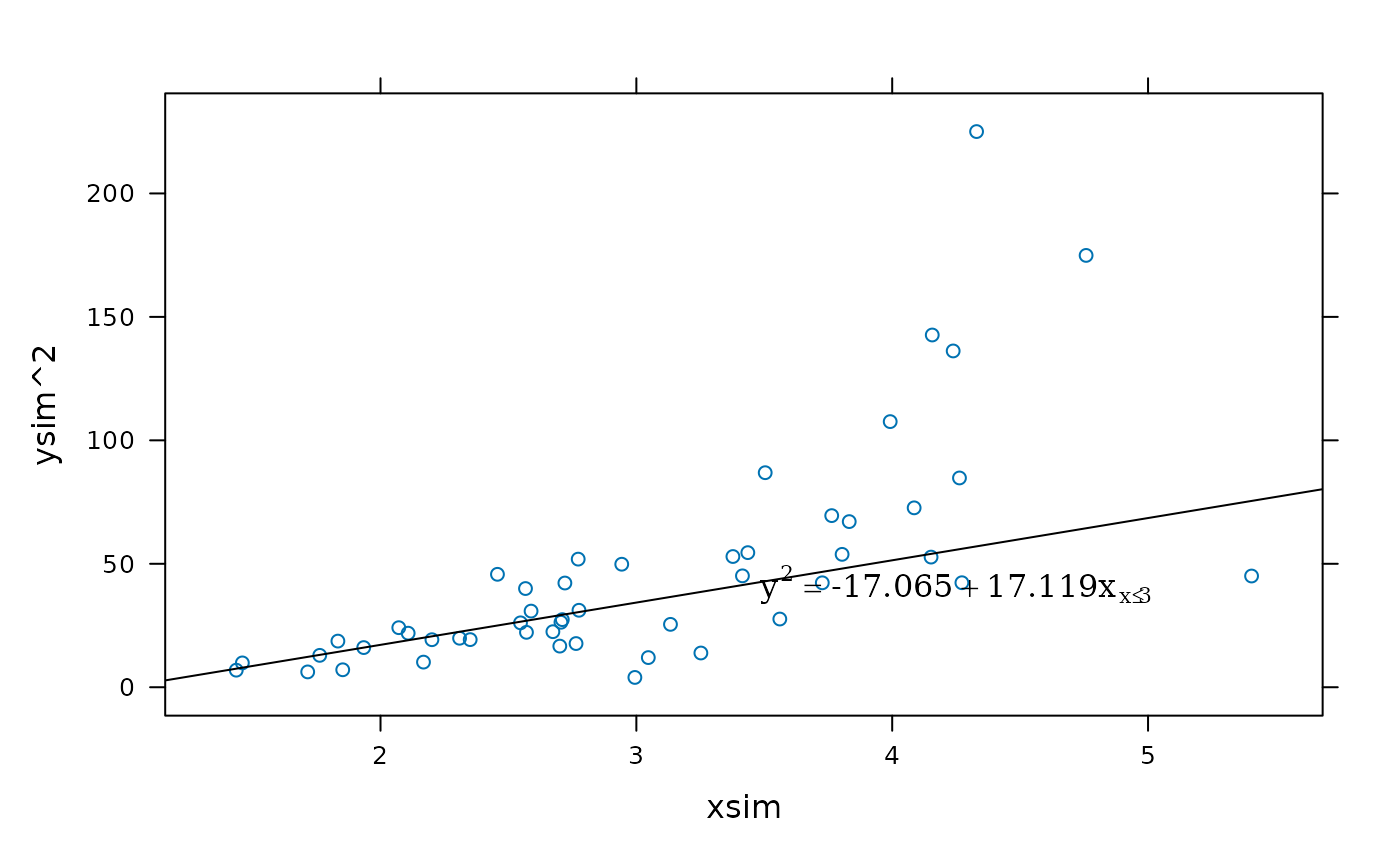
 ## using layers:
xyplot(ysim^2 ~ xsim) +
layer(panel.ablineq(lm(y ~ x, subset = x <= 3),
varNames = alist(y = y^2, x = x[x <= 3]), pos = 4))
## using layers:
xyplot(ysim^2 ~ xsim) +
layer(panel.ablineq(lm(y ~ x, subset = x <= 3),
varNames = alist(y = y^2, x = x[x <= 3]), pos = 4))
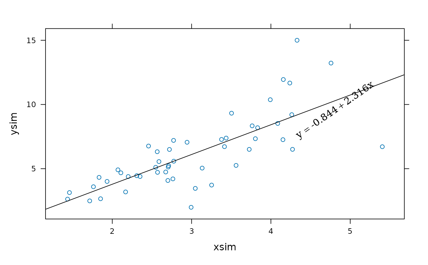
 ## rotated equation (depends on device aspect at plotting time)
xyplot(ysim ~ xsim) +
layer(panel.ablineq(lm(y ~ x), rotate = TRUE, at = 0.8))
## rotated equation (depends on device aspect at plotting time)
xyplot(ysim ~ xsim) +
layer(panel.ablineq(lm(y ~ x), rotate = TRUE, at = 0.8))
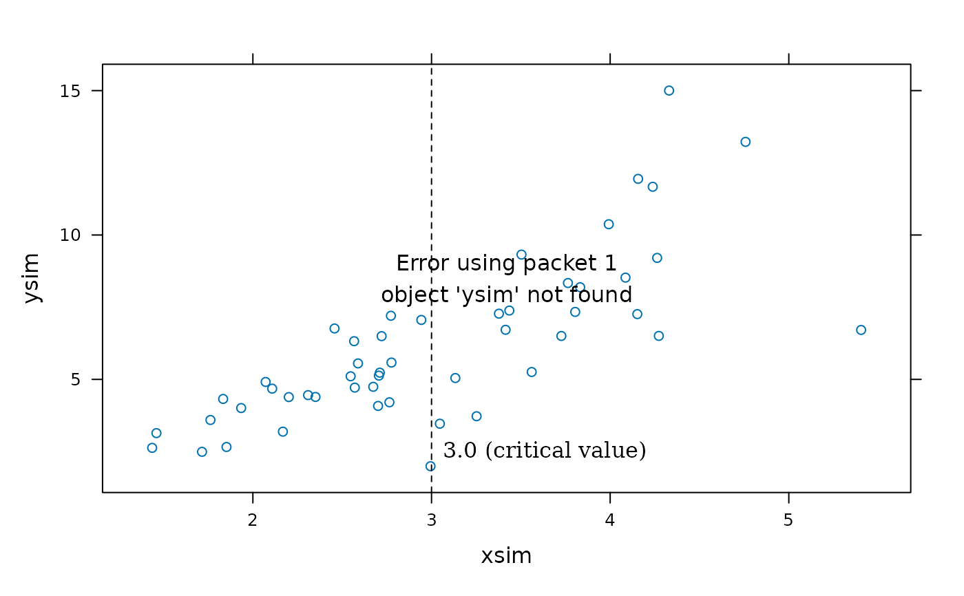
 ## horizontal and vertical lines
xyplot(ysim ~ xsim) +
layer(panel.ablineq(v = 3, pos = 4, at = 0.1, lty = 2,
label = "3.0 (critical value)")) +
layer(panel.ablineq(h = mean(ysim), pos = 3, at = 0.15, lty = 2,
varNames = alist(y = plain(mean)(y))))
## horizontal and vertical lines
xyplot(ysim ~ xsim) +
layer(panel.ablineq(v = 3, pos = 4, at = 0.1, lty = 2,
label = "3.0 (critical value)")) +
layer(panel.ablineq(h = mean(ysim), pos = 3, at = 0.15, lty = 2,
varNames = alist(y = plain(mean)(y))))
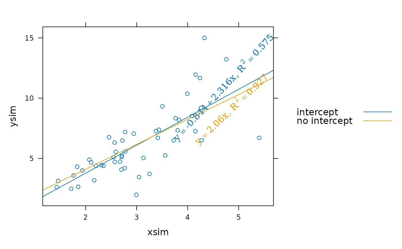
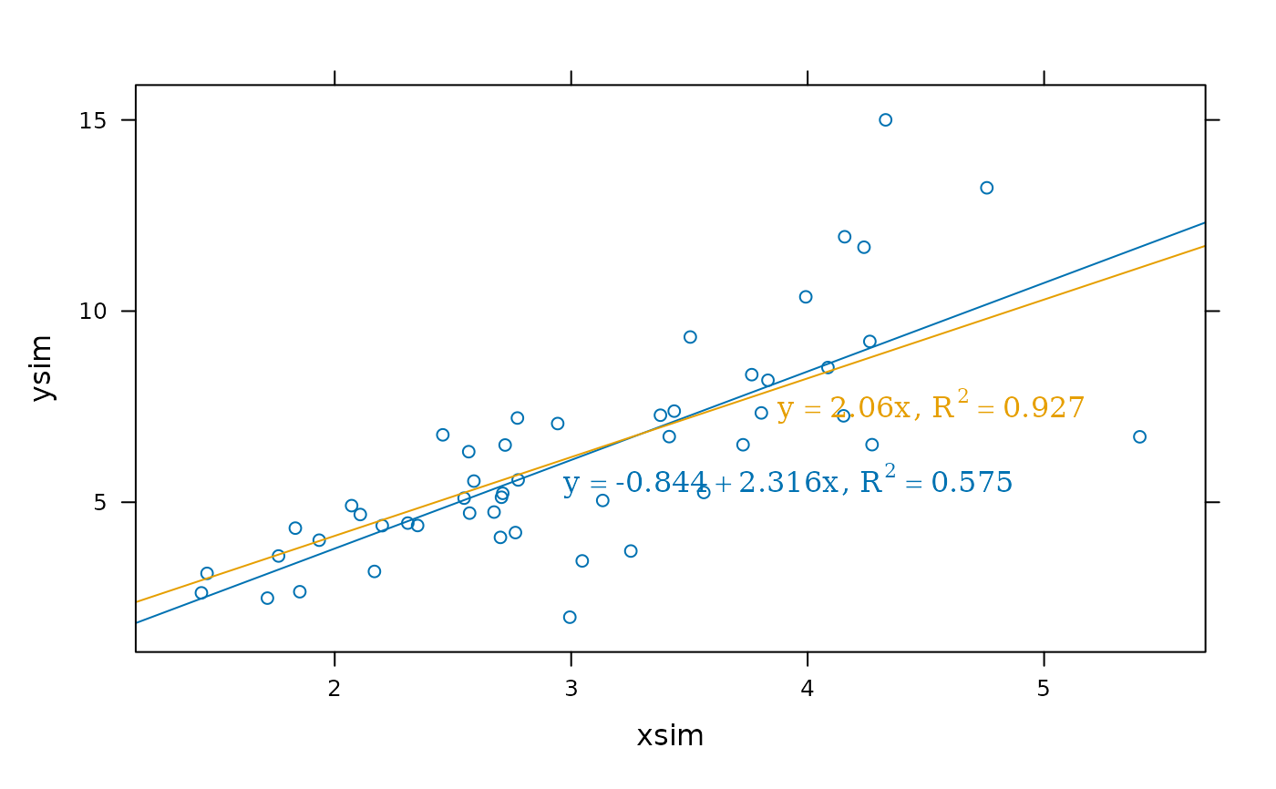
 ## using layer styles, r.squared
xyplot(ysim ~ xsim) +
layer(panel.ablineq(lm(y ~ x), r.sq = TRUE,
at = 0.4, adj=0:1), style = 1) +
layer(panel.ablineq(lm(y ~ x + 0), r.sq = TRUE,
at = 0.6, adj=0:1), style = 2)
## using layer styles, r.squared
xyplot(ysim ~ xsim) +
layer(panel.ablineq(lm(y ~ x), r.sq = TRUE,
at = 0.4, adj=0:1), style = 1) +
layer(panel.ablineq(lm(y ~ x + 0), r.sq = TRUE,
at = 0.6, adj=0:1), style = 2)
 ## alternative placement of equations
xyplot(ysim ~ xsim) +
layer(panel.ablineq(lm(y ~ x), r.sq = TRUE, rot = TRUE,
at = 0.8, pos = 3), style = 1) +
layer(panel.ablineq(lm(y ~ x + 0), r.sq = TRUE, rot = TRUE,
at = 0.8, pos = 1), style = 2)
## alternative placement of equations
xyplot(ysim ~ xsim) +
layer(panel.ablineq(lm(y ~ x), r.sq = TRUE, rot = TRUE,
at = 0.8, pos = 3), style = 1) +
layer(panel.ablineq(lm(y ~ x + 0), r.sq = TRUE, rot = TRUE,
at = 0.8, pos = 1), style = 2)
 update(trellis.last.object(),
auto.key = list(text = c("intercept", "no intercept"),
points = FALSE, lines = TRUE))
update(trellis.last.object(),
auto.key = list(text = c("intercept", "no intercept"),
points = FALSE, lines = TRUE))